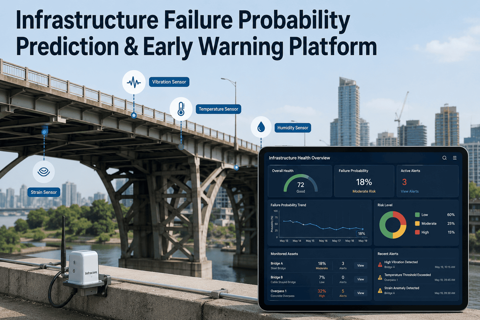
Infrastructure failure prediction has moved beyond rules-of-thumb and inspection calendars. Modern machine learning now detects developing structural and mechanical faults weeks to months before they reach functional failure — but the choice of model architecture decides whether predictions are precise enough to act on or just noise that erodes engineer trust. Random Forest dominates static condition scoring on bridges and slopes. LSTM and GRU networks own long-horizon time-series prognostics for pumps, motors, and pipelines. CNNs lead visual defect detection on rail, pavement, and concrete surfaces. XGBoost wins on imbalanced fault data. Transformers are reshaping multi-asset condition forecasting. And survival models (Weibull, Cox PH) remain the workhorse for asset cohorts where failure data is sparse. This deep dive maps each model family to the infrastructure problem it actually solves — and shows how a hybrid stack produces production-grade predictions. Book a Demo to see iFactory's multi-model engine running on live UK, EU, and MENA infrastructure.
0.97+
F1 score reached by Gradient Boosting on industrial fault classification
2-8 wks
Typical ML lead time before functional failure on rotating equipment
~50%
Of all rotating-machine breakdowns caused by bearing failures alone
70-80%
Of needed sensor data already captured by existing BAS and SCADA systems
Jump to a Model Family
01 · Random Forest
02 · Gradient Boosting (XGBoost)
03 · LSTM & GRU
04 · CNN (Visual)
05 · Transformers
06 · Survival Models
Model 01
Random Forest — Tabular Workhorse
Ensemble of decision trees voting on the final prediction. The most widely deployed model in civil infrastructure because it handles mixed data types, requires minimal tuning, and produces feature importance scores engineers can interpret directly.
Strongest On
Geotechnical hazards — slopes, embankments, retaining walls
Bridge condition rating classification from inspection records
Pavement distress probability from environmental and load factors
Datasets where explainability matters for regulatory review
Benchmark Evidence
AUC, F1, and accuracy of 1.0 on a transportation slope failure dataset
Top features ranked: elevation, distance to streams, NDVI, precipitation
Optimal probability threshold typically tuned to 0.65–0.75
Matches deep learning on simple, repetitive failure patterns
Trade-offCannot model temporal order. For week-long degradation trajectories, sequence models capture context that flattened features miss.
Model 02
Gradient Boosting (XGBoost / LightGBM) — Imbalanced Fault Champion
Trees built sequentially, each one correcting errors of the last. The default choice when failure events are rare relative to normal operation — exactly the case in infrastructure, where weeks of healthy data surround each fault.
Strongest On
Power transformer fault classification on imbalanced fault data
Water main break and pipeline leak probability scoring
Cloud and IT job failure prediction with feature importance
When SHAP explainability is needed for audit defence
Benchmark Evidence
F1 above 0.97 on industrial fault datasets
Top performer in cloud job failure studies (vs LR, DT, RF)
Handles class imbalance well — failures often under 5% of records
Trains on CPU; deployable on edge hardware
Trade-offTreats sequence as feature position rather than ordered evidence. Long-term temporal dependencies are not captured natively.
Model 03
LSTM & GRU — Time-Series Specialists
Recurrent networks that process data in sequence, remembering long-range patterns through gated cells. Where a threshold model sees one out-of-range reading, an LSTM sees a deterioration trend — and distinguishes real failure from operational noise.
Strongest On
Remaining Useful Life (RUL) estimation on rotating equipment
Multi-sensor degradation tracking on pumps, motors, compressors
Pipeline temperature, pressure, and flow forecasting
Anomaly detection on continuous SCADA telemetry
Benchmark Evidence
Outperforms tree models on complex, multi-variable sensor datasets
Lower MAE and RMSE on degradation regression tasks
Quantile LSTM variants give uncertainty bands for risk-aware scheduling
Bi-layer and tri-layer architectures common in production
Trade-offAccuracy decreases as the prediction window extends. For very long horizons, Transformers often surpass LSTM.
Model 04
CNN — Visual Defect Detection
Convolutional Neural Networks process image data through layered feature maps. The dominant architecture for any infrastructure problem where a camera, thermal sensor, or laser scan is the primary input.
Strongest On
Crack detection on bridge decks, tunnels, concrete structures
Pavement distress segmentation from drive-by imagery
Rail surface defect classification from line-scan cameras
Thermal anomaly detection on transformers and switchgear
Benchmark Evidence
Standard backbone for infrared scan analysis on transformer surfaces
YOLO and U-Net variants reach 90%+ mAP on defect segmentation
Transfer learning from ImageNet cuts training data needs sharply
Edge-optimised variants (MobileNet, EfficientNet) run on field hardware
Trade-offRequires labelled image data, which is expensive to produce. Robustness drops under lighting and weather conditions not seen in training.
Model 05
Transformer Architectures — Emerging State of the Art
Self-attention lets every element in a sequence reference every other element. For infrastructure, that means correlating today's vibration pattern with one from twelve months ago — capturing long-range dependencies that LSTMs struggle with.
Strongest On
Bridge condition forecasting from decades of inspection reports
Multi-modal data fusing sensor, image, and text inputs
Fault diagnosis on rotating machinery with rich vibration signatures
Variable-format inputs that defeat fixed-schema models
Benchmark Evidence
Treats inspection ratings as tokens — adapts to real-world variability
T4PdM Transformer benchmarked on MaFaulDa and CWRU bearing data
Compact 2-layer 4-head encoders outperform LSTM on long horizons
Increasingly favoured for multi-asset prognostics in 2025–26 research
Trade-offHighest data and compute cost in this guide. Overkill for simple patterns where Random Forest or XGBoost match accuracy.
Model 06
Survival Models (Weibull, Cox PH) — Sparse-Data Workhorse
Statistical models that estimate time-to-failure distributions from censored data. The best choice when failure events are rare or historical sensor data is incomplete — exactly the situation in legacy infrastructure portfolios.
Strongest On
Cohort-level RUL on bearings, transformers, valves
Capital planning where individual sensor data is unavailable
Wind turbine main bearing lifecycle modelling
High-voltage instrument transformer replacement planning
Benchmark Evidence
Weibull β shape parameter distinguishes early, random, and wear-out failures
Combined Weibull + neural net achieves accurate bearing RUL
Used by TenneT for transmission-grid maintenance scenario simulation
Works with as few as 30–50 lifecycle observations per asset class
Trade-offAssumes a parametric failure distribution. Less precise than data-driven models when rich sensor history is available.
At-a-Glance Benchmark Comparison
Choose your model based on data shape, horizon, and explainability needs. iFactory's pipeline orchestrates all six — automatically routing each task to the family that performs best.
Model
Data Type
Horizon
Explainability
Compute Cost
Random Forest
Tabular
Short
High
Low
XGBoost / LightGBM
Tabular (imbalanced)
Short to medium
High (SHAP)
Low
LSTM / GRU
Time-series
Medium
Medium
High
CNN
Image / spatial
Snapshot
Medium (Grad-CAM)
High
Transformer
Long sequences, multi-modal
Long
Lower
Very high
Survival (Weibull, Cox)
Censored lifecycle
Long
High
Very low
How iFactory Combines All Six in One Production Pipeline
In real deployments, no single model wins. iFactory routes each prediction task to the architecture that performs best for that asset class and data shape — and the pipeline stages cascade.
Stage 1
Anomaly Detection
Isolation Forest + Autoencoders
Stage 2
Fault Classification
XGBoost + Random Forest
Stage 3
RUL Estimation
LSTM + Quantile Regression
Stage 4
Long-Range Forecast
Transformer + Weibull
iFactory Infrastructure AI Platform
Don't Pick One Model. Deploy a Pipeline That Picks the Right One Automatically.
iFactory orchestrates Random Forest, XGBoost, LSTM, CNN, Transformer, and survival models in a single hybrid stack — already deployed on live infrastructure networks across the UK, EU, and MENA.
Trusted by infrastructure operators managing bridges, rail, water, energy, and transport networks.
Frequently Asked Questions
Tap any question to reveal the answer.
No single model wins everywhere. Research on multivariate industrial time-series shows LSTM significantly outperforms Random Forest and Logistic Regression on complex datasets with diverse failure patterns, while Random Forest matches or beats deep learning on simpler, repetitive patterns. The right answer is almost always a hybrid pipeline that routes each task to the most suitable architecture. Book a demo to see iFactory's hybrid stack in production.
For most facility and infrastructure use cases, tree-based models (Random Forest, XGBoost) handle 60–70% of predictions effectively — and remain easier to explain, faster to train, and cheaper to deploy. Deep learning becomes essential for long-range temporal dependencies (LSTM, Transformer), visual defect detection (CNN), or RUL regression with uncertainty bands. Start simple. Add deep learning where it measurably improves accuracy.
Anomaly detection (Isolation Forest, Autoencoders) deploys with 30–60 days of healthy operation — no labelled failures needed. Supervised classification typically needs 12 months of historical data with documented failure events. LSTM and Transformer models benefit from 2–3 years to capture seasonal patterns and rare faults. Roughly 70–80% of needed sensor data is usually already captured in existing BAS and SCADA systems.
Survival models (Weibull, Cox proportional hazards) are the right choice when failure data is sparse, individual sensor history is unavailable, or you need cohort-level remaining-life estimates for capital planning. Wind turbine bearings and high-voltage instrument transformers are textbook examples — both have well-documented Weibull-based RUL studies in production use. When rich sensor data is available, data-driven models typically outperform survival models on individual-asset precision.
iFactory's pipeline monitors accuracy continuously, benchmarking model output against confirmed field outcomes each month. Retraining triggers automatically when precision drops below the validated deployment baseline. Network change events — new sensors, asset additions, operational mode shifts — trigger out-of-cycle reviews. Every model version is logged with training data scope and accuracy metrics, providing the audit trail required for safety-critical infrastructure decisions.
Yes — with model selection awareness. Random Forest, XGBoost, and survival models run comfortably on CPU-only edge devices and are the standard for remote SCADA installations. Compact LSTM models (1–2 layers, modest hidden size) and edge-optimised CNNs (MobileNet, EfficientNet) also deploy at the edge. Full Transformer architectures typically need GPU or are reserved for cloud-tier processing. iFactory's deployment automatically distributes inference between edge and cloud based on latency requirements and connectivity.
Yes. Tree-based models offer native feature importance, and SHAP values explain individual predictions in both Random Forest and XGBoost. CNNs use Grad-CAM heatmaps to show which image regions drove a defect classification. Survival models are statistically transparent by construction. Transformers are the hardest to explain, which is why iFactory uses them selectively and pairs them with simpler models for any safety-critical decision that must be audit-defended.