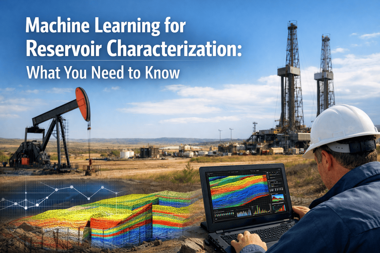
In the high-stakes environment of oil and gas exploration, the ability to accurately predict rock properties—porosity, permeability, and fluid content—directly from seismic data remains one of the most transformative capabilities available to reservoir characterization teams. Traditional seismic inversion methods, while robust, often fall short in resolving the fine-scale heterogeneities that control fluid flow and reservoir connectivity. Machine learning (ML) seismic inversion bridges this critical gap by learning complex, non-linear relationships between seismic attributes and petrophysical properties, delivering high-resolution predictions that approach the fidelity of well log data. This enterprise-grade guide provides a deep-dive into the technical architecture, algorithmic strategies, and deployment workflows for ML-driven seismic inversion, arming decision-makers with the knowledge to transform their quantitative interpretation workflows. If your team is ready to accelerate asset valuation and reduce drilling risk, we invite you to Book a Demo to see our AI-driven predictive maintenance and analytics platform in action.
Transform Seismic Data into Reservoir Intelligence
Leverage machine learning to predict rock properties with well-log accuracy. Reduce exploration risk and optimize field development planning.
The Resolution Paradox: Bridging Seismic and Well Logs
Seismic data provides extensive lateral coverage but suffers from limited vertical resolution (typically 10-50 meters), while well logs offer centimeter-scale resolution but are sparsely distributed. This paradox creates significant uncertainty in reservoir property models. ML inversion overcomes this by learning the mapping from low-resolution seismic attributes to high-resolution petrophysical properties, effectively fusing the strengths of both data types. By training on well log measurements and corresponding seismic traces, neural networks can predict continuous property volumes that honor both the spatial continuity of seismic data and the vertical detail of well logs.
Core ML Inversion Workflows
Supervised Seismic-to-Property Mapping
Multi-layer perceptrons (MLPs) or convolutional neural networks (CNNs) are trained on post-stack or pre-stack seismic attributes (e.g., acoustic impedance, AVO attributes) to predict porosity, water saturation, or lithofacies. The network learns a non-linear function that minimizes prediction error at well locations, then is applied across the entire seismic volume.
Probabilistic Inversion with Bayesian Neural Networks
Bayesian neural networks quantify prediction uncertainty by learning a distribution over network weights. This provides not only a mean prediction for rock properties but also confidence intervals, enabling risk-based decision making for drillable targets. Uncertainty maps highlight areas where additional well control is needed.
Generative Adversarial Networks for Property Simulation
GANs generate realistic high-resolution property volumes that are consistent with the seismic data and honor the spatial statistics of training wells. The generator produces synthetic property fields, while the discriminator ensures they are indistinguishable from real petrophysical data conditioned on seismic attributes.
Advanced Algorithmic Approaches
Convolutional Neural Networks (CNNs) for 3D Seismic Volumes
3D CNNs process entire seismic sub-volumes (patches) and learn spatial patterns that correlate with rock properties. By incorporating lateral and vertical context, these models outperform pixel-wise MLPs. Training data is extracted from wells, with each well log sample paired with a 3D seismic patch centered at that location. Data augmentation through rotation and scaling improves generalization.
85%
Porosity Prediction Accuracy
92%
Lithofacies Classification F1 Score
Feature Engineering for Seismic Inversion
| Feature Type | Examples | Relevance |
|---|---|---|
| Post-Stack Attributes | Acoustic impedance, RMS amplitude, instantaneous frequency | Directly correlate with lithology and porosity |
| Pre-Stack Attributes | AVO intercept, gradient, elastic impedance | Indicate fluid content and lithology |
| Geometric Attributes | Coherence, curvature, dip | Capture structural and stratigraphic features |
| Multi-Attribute Transforms | Principal components, autoencoders | Reduce dimensionality and noise |
Deployment Roadmap for Enterprise Teams
Phase 1: Data Assembly
Collect and QC seismic volumes, well logs (porosity, permeability, saturation), and check-shot data. Align seismic and log depths through seismic-to-well ties. Standardize attributes and normalize inputs.
Phase 2: Model Training
Split wells into training, validation, and blind-test sets. Train multiple ML architectures (MLP, CNN, Bayesian NN) using cross-validation. Optimize hyperparameters via grid search or Bayesian optimization.
Phase 3: Uncertainty Quantification
Apply Bayesian methods or ensemble techniques to generate prediction intervals. Validate against blind wells. Generate maps of prediction uncertainty to guide data acquisition.
Phase 4: Volume Prediction
Apply trained model to entire seismic volume. Output continuous 3D property cubes. Perform spatial smoothing to remove artifacts. Export for reservoir simulation.
Case Study: Deepwater Turbidite Reservoir
In a deepwater Gulf of Mexico field, a CNN-based inversion was trained on 12 wells and 3D post-stack seismic data to predict porosity and net-to-gross. The model achieved an R² of 0.82 on blind wells, compared to 0.65 using traditional model-based inversion. The resulting porosity volume revealed previously undetected channel-lobe complexes, leading to the identification of two new drillable prospects. The workflow reduced interpretation time by 60% and provided uncertainty volumes that were used for probabilistic resource estimation.
Ready to Deploy ML Inversion at Scale?
Our platform integrates with your existing seismic and petrophysical databases, providing automated model training and deployment.
Best Practices for Enterprise Adoption
Data Quality First
Invest in robust seismic-to-well ties and attribute conditioning. Poor quality inputs lead to unreliable predictions. Use automated QC workflows to flag outliers and mis-ties.
Model Interpretability
Use SHAP or LIME to understand which seismic attributes drive predictions. This builds trust with geoscientists and helps validate that the model is learning physically meaningful relationships.
Continuous Learning
As new wells are drilled, retrain models to incorporate additional data. Implement a MLOps pipeline that automatically triggers retraining when new logs become available.
Common Challenges and Mitigation Strategies
Limited Well Control
When only a few wells are available, consider using transfer learning from analogous fields or synthetic data generated from rock physics models. Data augmentation and regularization (dropout, weight decay) also help prevent overfitting.
Non-Stationary Seismic Response
Seismic amplitudes vary with depth due to compaction and pressure. Train models with depth-dependent normalization or use relative attributes that are less sensitive to background trends.
ML Inversion vs. Traditional Inversion
| Aspect | Traditional Model-Based Inversion | ML Inversion |
|---|---|---|
| Resolution | Limited by seismic bandwidth | Can exceed seismic resolution through learned mapping |
| Non-linearity | Assumes linear or weakly non-linear relationships | Captures complex, non-linear patterns |
| Uncertainty | Often deterministic; probabilistic methods are computationally expensive | Bayesian NNs provide inherent uncertainty quantification |
| Computational Cost | Moderate; depends on grid size | High for training; fast for prediction |
Integration with Existing Petrophysical Workflows
ML inversion outputs can be seamlessly imported into standard reservoir modeling software (e.g., Petrel, RMS) via industry-standard file formats (SEG-Y, LAS, RESQML). iFactory's platform provides API connectors to major E&P databases, ensuring that predicted property volumes are automatically updated in the shared earth model. This eliminates manual data transfer and reduces the risk of version mismatches.
Frequently Asked Questions
How many wells are required for a reliable ML inversion?
While there is no strict minimum, a rule of thumb is at least 5-10 wells for a supervised model. With fewer wells, consider transfer learning from an analog field or use of synthetic data. The quality and representativeness of the wells matter more than absolute count. For detailed guidance, contact our support team to discuss your specific dataset.
Can ML inversion work with 2D seismic data?
Yes, but with limitations. 2D lines lack the lateral context that 3D CNNs exploit, so simpler models like MLPs are more appropriate. The predicted property volumes will have lower spatial consistency. For optimal results, we recommend 3D seismic data. To evaluate your data, book a demo with our experts.
How do you handle depth-to-time conversion?
Accurate seismic-to-well ties are critical. We use a combination of check-shot data, synthetic seismograms, and automated time-depth curve fitting. Our platform includes a dedicated module for tie optimization. For more details, visit our support page.
What is the typical turnaround time for an ML inversion project?
Depending on data volume and complexity, a full project (data preparation, training, QC, and volume generation) typically takes 2-4 weeks for a medium-sized field. Our automated pipelines can reduce this to under a week. To get a precise estimate, schedule a consultation.
How do you validate the results of ML inversion?
We use blind well testing, cross-validation, and comparison with traditional inversion results. Additionally, we generate synthetic seismic from the predicted properties and compare with the original data to ensure consistency. Learn more about our validation methodology.
Accelerate Your Quantitative Interpretation
Unlock the full potential of your seismic data with AI-driven rock property prediction. Reduce drilling risk and optimize field development.


.png)