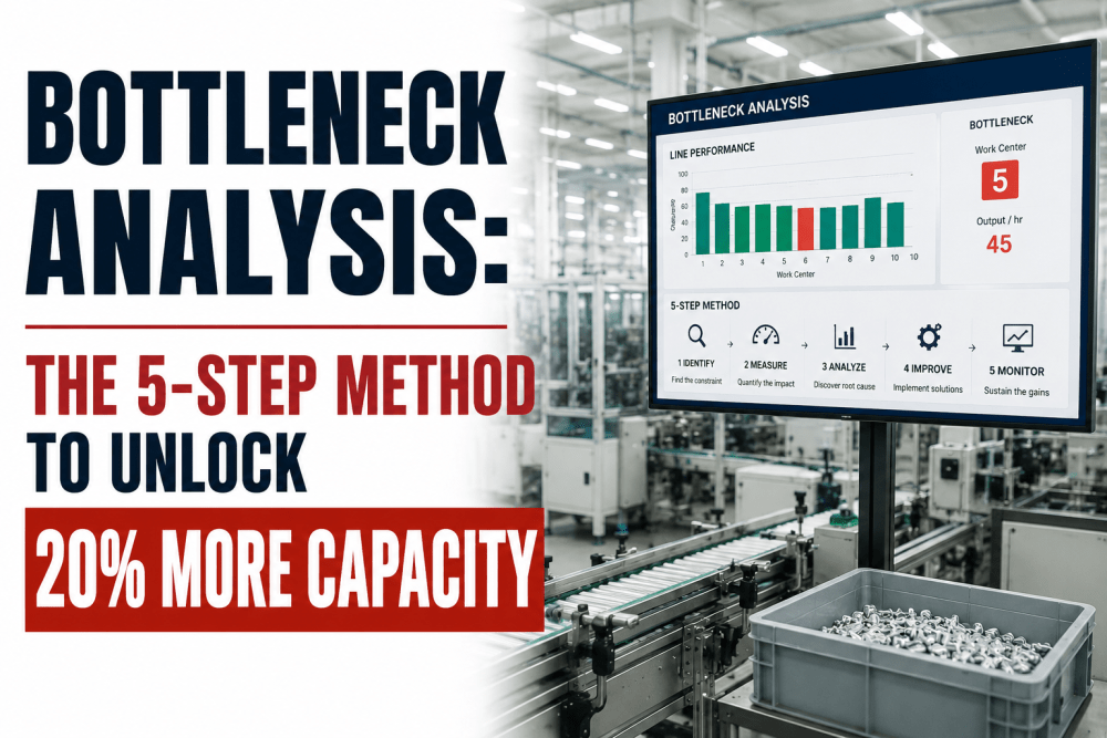
Bottleneck Analysis: The 5-Step Method to Unlock 20% More Capacity
By Daniel Brooks on May 23, 2026
Bottleneck analysis is one of the most consequential methods a manufacturing operation can apply — not because it's complicated, but because it answers the one question that drives every capacity and throughput conversation: where exactly is this plant leaving production capacity on the table? A factory running 20% below its rated output is not uniformly underperforming across every machine and workstation. It is being constrained by one or two specific assets, processes, or workflows that are limiting the entire system's throughput. Identifying those constraints, quantifying their cost and eliminating them in sequence is the structured practice of bottleneck analysis. This guide covers the five-step method that U.S. manufacturers are using in 2026 to unlock 15–25% additional capacity — from constraint identification through digital twin simulation and sustained throughput improvement.
Digital Twin Simulation · iFactory AI
Find Your Bottleneck in 72 Hours
iFactory's Digital Twin platform connects to your existing PLC and MES data to identify your system constraint, quantify the throughput cost, and model every proposed fix — before a dollar of capital is committed.
What Is a Manufacturing Bottleneck — and Why Most Plants Misidentify Theirs
A bottleneck is any resource — machine, workstation, operator station, or process step — whose capacity is less than or equal to the demand placed on it, causing work-in-progress to accumulate upstream and starving downstream operations of material. The critical distinction: a bottleneck is not simply the slowest step in a process. It is the step that limits the throughput of the entire system. In complex multi-stage manufacturing lines, a slow machine that is never fully loaded is not the bottleneck. A machine running at 97% utilization that causes queue buildup every time a downstream changeover occurs is.
Constraint Type 1
Capacity Bottleneck
A physical asset or workstation whose maximum throughput rate is lower than the demand placed on it by the production schedule. The most common type — typically a single machine, press, oven, or inspection station that cannot process parts fast enough to keep downstream operations fed.
Capacity bottlenecks cause 60–70% of all unplanned throughput losses in discrete manufacturing
Constraint Type 2
Policy Bottleneck
A production rule, scheduling logic, or management policy that restricts throughput below what the physical assets could deliver. Batch release rules, quality hold procedures, shift patterns that don't align with demand, and over-restrictive setup approval workflows all create policy bottlenecks that are invisible in capacity planning models.
Policy bottlenecks account for 18–28% of preventable throughput losses in U.S. plants
Constraint Type 3
Material Bottleneck
A supply, inventory, or logistics constraint that starves the production system of the inputs it needs to run at capacity. Can appear as a supplier lead time issue, internal staging failure, or WIP imbalance between production stages — often misdiagnosed as a capacity problem when the fix is a scheduling or inventory positioning change.
Material bottlenecks are the fastest to resolve once correctly identified — average 14–21 day correction cycle
The 5-Step Bottleneck Analysis Method
The following five-step method is grounded in Eliyahu Goldratt's Theory of Constraints (TOC) and extended with real-time data analytics and digital twin simulation capabilities that were not available when TOC was first formalized. Each step builds on the previous — skipping steps, particularly Step 2, is the most common reason bottleneck analysis programs stall without producing throughput gains.
Step 1
Map the Value Stream and Collect Process Rate Data
Before any constraint can be identified, the complete process flow must be mapped with actual cycle times, setup times, and available capacity data at every stage — not theoretical rates from equipment spec sheets. Pull production data from PLC historians, MES records, and OEE systems to establish actual throughput rates per station per shift. Include material handling time, quality inspection dwell time, and batch transfer delays. Value stream maps built from engineering standards rather than actual runtime data routinely misidentify the bottleneck by 1–3 process steps.
Output: Current-state value stream map with actual cycle times, utilization rates, and WIP queue sizes at each stage
Step 2
Identify the Constraint Using WIP Accumulation and Utilization Data
The true bottleneck is identified by two converging signals: WIP queue accumulation immediately upstream (material piling up before this station) and downstream starvation (subsequent operations waiting for material). Utilization data alone is insufficient — a machine at 95% utilization that is never queue-constrained is not the bottleneck. Cross-reference utilization percentages against WIP queue depth trends over a 30-day rolling period. In plants with real-time OEE dashboards, the bottleneck station typically stands out within 72 hours of data analysis. In plants relying on manual data collection, the identification process takes 2–4 weeks and often produces incorrect results.
Output: Confirmed constraint station with quantified queue accumulation rate and downstream starvation frequency
Step 3
Exploit the Constraint — Maximize Output Without Capital Spend
Before investing in additional capacity, the TOC discipline requires exhausting every method of extracting more throughput from the existing constraint. Exploitation tactics include: eliminating non-value-added time at the bottleneck (changeover time, material wait time, quality re-inspection); dedicating skilled operators to the constraint station; shifting scheduled maintenance on the constraint to weekends or planned downtime windows; and removing quality inspection steps from the bottleneck that can be performed upstream or downstream without affecting yield. In most plants, exploitation of the constraint alone recovers 8–15% of rated throughput before any capital is spent.
Output: Constraint exploitation plan with projected throughput recovery, assigned ownership, and 30-day implementation timeline
Step 4
Subordinate All Other Processes to the Constraint
Every non-bottleneck process in the plant should be scheduled and operated to support the constraint — not to maximize its own local efficiency. This means upstream operations should pace their output to feed the constraint at its optimal rate, not faster. Running upstream processes at maximum speed to maximize their individual OEE scores builds excess WIP inventory, increases material handling costs, and adds no throughput because the constraint cannot process the material any faster. Subordination requires resetting scheduling logic in the MES and managing shift supervisors who have historically been measured on local utilization targets rather than system throughput.
Output: Revised production scheduling logic that subordinates non-constraint operations to the system constraint rate
Step 5
Elevate the Constraint and Repeat the Cycle
If exploitation and subordination have fully utilized the constraint but throughput is still insufficient, capital investment to elevate the constraint's capacity is now justified — because Steps 3 and 4 have proven that the constraint is genuinely limiting the system rather than being artificially underutilized. After elevation, the constraint will shift to a different station. The five-step cycle must restart immediately with the new constraint identified and characterized. Plants that treat bottleneck analysis as a one-time project rather than a continuous improvement cycle plateau within 18–24 months and lose the throughput gains they achieved in the first improvement cycle.
Output: Elevated constraint capacity, identified next system constraint, continuous improvement cycle restarted with updated value stream data
Bottleneck Analysis by Industry: Where Constraints Hide
Bottlenecks manifest differently across manufacturing sectors based on process architecture, product mix complexity, and the nature of the production system. The profiles below reflect where real constraints are typically found — and frequently misdiagnosed — in four major U.S. manufacturing segments.
Discrete Manufacturing · Constraint Profile
Primary Constraint: Machine Capacity at High-Value Processing Steps
In discrete manufacturing (machined components, fabricated metal, electronics assembly), the constraint is most often a CNC machining center, press, or automated assembly station that handles the highest-complexity or tightest-tolerance operations. These stations accumulate WIP because they cannot be substituted — the specific tooling, fixture, or programming capability is unique to that asset. Setup time reduction at the constraint station is the fastest exploitation tactic, often recovering 12–18% of effective capacity without any capital investment.
68–74%Typical constraint utilization before analysis
12–18%Capacity recovered through setup time reduction alone
Setup TimePrimary exploitation lever at the constraint
Food & Beverage · Constraint Profile
Primary Constraint: Packaging and Filling Lines at Peak SKU Count
Food and beverage plants typically run highest constraint utilization on filling and packaging lines during high-SKU-count production periods. The constraint shifts dynamically with product mix — a line configured for 12 oz retail packs may run at 91% utilization while a 1-gallon format runs at 62%. Bottleneck analysis in this environment requires constraint identification by SKU family, not just aggregate line utilization. Changeover time between formats is invariably the primary exploitation target, with SMED methodology delivering 25–40% changeover time reductions in well-executed programs.
SKU-DependentConstraint shifts with product mix changes
25–40%Changeover time reduction through SMED at the constraint
ChangeoverPrimary exploitation lever for packaging constraints
Automotive Supplier · Constraint Profile
Primary Constraint: Stamping or Welding Operations on High-Volume Components
Tier 1 and Tier 2 automotive suppliers most often find their system constraint at a stamping press, robotic welding cell, or heat treatment furnace. These operations typically have long cycle times, high tooling costs that make parallel capacity expensive, and strict quality requirements that add inspection time at the constraint. The policy bottleneck risk is elevated in automotive environments — quality hold procedures, PPAP approval requirements, and customer-specific inspection intervals frequently add 15–22% of non-value-added time at the physical constraint, making policy bottleneck elimination critical before capital elevation is considered.
15–22%Non-value-added time from policy constraints at the bottleneck
Stamping / WeldingMost common physical constraint locations
Policy + CapacityDual constraint type — resolve policy before elevating capacity
Pharmaceuticals · Constraint Profile
Primary Constraint: Quality Testing and Batch Release Procedures
Pharmaceutical manufacturing is the sector where policy bottlenecks most consistently outweigh physical capacity constraints. In-process testing hold times, batch record review cycles, QA release approval workflows, and environmental monitoring sampling schedules routinely constrain throughput more severely than any physical processing step. A granulation suite or tablet press running at 58% utilization may appear to be the constraint — but the root cause is a 72-hour batch release hold that accumulates WIP upstream and starves downstream packaging. Identifying and restructuring the batch release workflow is the highest-leverage bottleneck intervention in most pharmaceutical plants.
Batch ReleaseMost frequent constraint type — policy, not physical capacity
20–35%Throughput gain from policy restructuring before capital spend
Quantifying the Cost of Your Bottleneck: The Throughput Loss Waterfall
The most effective way to build organizational alignment around bottleneck elimination — and justify the analytics investment required to do it precisely — is a throughput loss waterfall that converts constraint data into dollar terms. The example below is representative of a mid-size discrete manufacturer at 850,000 units per year rated capacity running a 5-stage production line.
Rated Annual Capacity
850,000 units/yr · 100%
Planned Maintenance & Changeover
−7%
Bottleneck Station Unplanned Downtime
−12%
Speed / Feed Rate Losses at Constraint
−8%
Policy & Scheduling Losses (Non-Physical)
−6%
Actual Annual Output
569,500 units/yr · 67%
Target After Bottleneck Elimination (18 Months)
714,000 units/yr · 84%
Improvement opportunity: 144,500 additional units per year · ~$7.2M incremental revenue at $50/unit contribution margin
Most manufacturers report 80–85% efficiency while their true throughput is 65–72% of rated capacity. The gap is in the bottleneck — and it's measurable.
iFactory's Digital Twin simulation platform maps your production constraints in real time, quantifies the throughput impact of each bottleneck, and models the outcome of every proposed intervention before a dollar of capital is committed.
The precision and speed of bottleneck identification depends directly on the quality of the tooling used to collect and analyze process data. The comparison below reflects the functional difference between manual analysis methods, basic MES reporting, and a real-time digital twin platform with integrated constraint analytics.
Capability
Manual / Spreadsheet Analysis
Standard MES Reporting
Digital Twin Platform (iFactory)
Operational Impact
Constraint Identification Speed
2–6 weeks of manual data collection
3–10 days with report extraction
48–72 hours from data connection
Faster identification = fewer lost production days before intervention
WIP Queue Tracking
Manual observation only — snapshot data
End-of-shift batch totals
Real-time queue depth with trend visualization
Dynamic bottleneck shifting captured vs. missed in batch reporting
Constraint Type Classification
Engineering judgment — high error rate
Limited — capacity data only
Automated: capacity, policy, and material constraint flags
Correct constraint type determines correct intervention — misclassification wastes capital
Intervention Modeling
None — estimates only
Static what-if scenarios only
Digital twin simulation of proposed changes before implementation
Validate throughput gain before capital commitment — eliminates failed improvement projects
Downstream Starvation Detection
Manual — observed during floor walks
Utilization reporting — indirect signal
Automatic starvation event logging with duration and cost
Identifies true constraint vs. slow station misidentification
Constraint Shift Detection
Not detected — requires new analysis cycle
Requires manual re-analysis
Automatic constraint migration alerts when bottleneck moves
Prevents improvement investment in a station that is no longer the constraint
ROI Calculation
Manual — often overstated by 40–60%
Partial — based on throughput data only
Automated: throughput, labor, energy, and inventory cost model
Accurate business case for capital elevation decisions
Digital Twin Simulation: Modeling Constraint Elimination Before Committing Capital
The highest-value application of digital twin technology in bottleneck analysis is intervention validation — running every proposed change through a simulation model before implementation to confirm that the projected throughput gain is real and that the intervention does not simply shift the constraint to a new, more expensive location. This section covers how the simulation workflow integrates with the five-step TOC method.
01
Build the Digital Twin from Live Production Data
The digital twin is constructed from actual production data — PLC cycle times, OEE records, MES scheduling data, and historical downtime logs — not from engineering specifications. The model is validated against 90 days of actual production output before any simulation scenario is run. A digital twin calibrated to real performance data typically predicts throughput outcomes within 3–5% of actual results. A twin built from design parameters diverges by 15–25% and produces unreliable intervention projections.
02
Simulate the Exploitation Scenarios (No Capital)
Before modeling capital investments, simulate every zero-cost exploitation tactic identified in Step 3: setup time reduction at the constraint, elimination of non-value-added inspection time, operator allocation changes, and scheduling sequence optimization. The simulation quantifies the throughput gain from each tactic individually and in combination, allowing the improvement team to identify the minimum intervention set that achieves the target throughput — before deciding whether capital elevation is necessary at all.
03
Identify Constraint Migration Risk
Every simulation run that successfully elevates the current bottleneck immediately reveals where the next constraint will appear. This is the critical insight that manual bottleneck analysis cannot provide — when a plant invests $1.2M to add capacity at its current bottleneck, only to discover that the next constraint surfaces at a $3.8M asset that was not in the capital plan, the project delivers far less throughput gain than projected. The digital twin maps the full constraint migration cascade before the first dollar of investment is approved.
04
Generate the Capital Investment Sequence
The simulation output produces a ranked investment sequence — the order in which bottleneck elevations deliver the highest throughput gain per dollar of capital committed. This sequence typically differs from the intuitive priority order that operations teams derive from floor observation. Plants that implement capital investments in simulation-validated sequence consistently achieve 22–31% higher throughput gains per dollar invested compared to plants that sequence investments based on engineering judgment alone.
05
Validate in Production and Update the Twin
After each intervention is implemented, actual production results are compared against the simulation prediction. Divergences — when the real plant behaves differently from the twin — are used to update and improve the model. Over 3–5 improvement cycles, the digital twin becomes increasingly accurate and the validation gap between predicted and actual throughput gain narrows to under 2%. This accumulating accuracy is why plants with mature digital twin programs consistently outperform their improvement targets while plants relying on periodic bottleneck studies repeatedly underdeliver.
Expert Review: Bottleneck Analysis in U.S. Manufacturing Operations
OM
Operations Management Perspective
Compiled from manufacturing operations and industrial engineering reviews across U.S. discrete and process manufacturing facilities
What consistently delivers results
Starting the analysis at the constraint's downstream neighbor, not at the constraint itself. The downstream starvation signature — an operation frequently idle waiting for material — is the clearest and most unambiguous indicator of the true bottleneck location. Starting with the station that appears busiest leads to misidentification in roughly 40% of initial assessments.
Measuring constraint utilization at 5-minute intervals rather than shift averages. A constraint station averaging 78% utilization across a shift may be running at 97% for 4-hour blocks and at 45% during material wait periods. The average hides the blocking behavior. Interval data reveals it, and the blocking pattern identifies whether the root cause is the constraint itself or a feeding process that is intermittently starving it.
Treating setup time reduction at the constraint as a financial project, not a process improvement project. Quantifying setup time as a dollar-per-hour cost — using the actual throughput contribution of the constraint station — consistently accelerates internal approval and resource allocation for SMED programs by framing the improvement in terms management already tracks.
Confirming that the bottleneck has actually moved before beginning a new improvement cycle. The most common failure mode in mature bottleneck analysis programs is continuing to invest in the original constraint after exploitation and subordination have shifted the system constraint to a new location. A monthly constraint confirmation run — 48 hours of WIP queue monitoring — prevents this misallocation.
Where analysis programs stall
Skipping subordination and jumping directly to constraint elevation. Plants that invest in additional capacity at the bottleneck without first ensuring that non-bottleneck processes are paced to the constraint rate routinely achieve only 30–50% of the projected throughput gain — because the new capacity immediately gets blocked or starved by the uncoordinated scheduling logic upstream and downstream.
Using aggregate production data rather than station-level interval data for constraint identification. A plant-level throughput number of 72% capacity cannot tell you where the bottleneck is. A WIP queue depth trend by station over a 30-day rolling window almost always can. The quality of the input data determines whether the bottleneck is correctly identified on the first analysis cycle or after a 3-month misdirected improvement effort.
Treating bottleneck analysis as a capital justification exercise rather than a continuous improvement cycle. Organizations that initiate a bottleneck study specifically to justify a pre-selected capital investment routinely misidentify the constraint, confirm their predetermined conclusion, and then express surprise when the capital project delivers below-forecast throughput improvement. The analysis must precede and drive the investment decision, not follow it.
The average U.S. manufacturer has $3M–$9M of annual throughput capacity sitting in unaddressed bottlenecks — across assets they already own.
iFactory's Digital Twin simulation platform identifies your system constraint within 72 hours of data connection, quantifies the throughput opportunity, and models every proposed intervention before implementation — so your capital goes to the right constraint, in the right sequence, with validated ROI.
Conclusion: Bottleneck Analysis Is a Revenue Decision, Not an Engineering Exercise
The manufacturers consistently running at 82–88% of rated capacity in 2026 are not operating fundamentally different equipment than those running at 65–70%. They have the same presses, the same machining centers, the same assembly lines. What they have is a structured, continuous practice of identifying where their system constraint is, extracting maximum throughput from that constraint before committing capital, and validating every improvement with data before and after implementation.
For a mid-size manufacturer with $50M in annual revenue and a 67% throughput realization rate, closing that gap to 84% represents $12.75M in additional revenue potential from the same plant, the same workforce, and the same equipment. Bottleneck analysis does not create new capacity — it recovers the capacity that already exists but is currently being blocked, starved, or misallocated by constraints that remain invisible without the right data infrastructure. The question is not whether the opportunity is worth pursuing. It is how quickly the right constraint visibility, simulation tooling, and improvement process can be put in place to start capturing it.
Frequently Asked Questions
OEE improvement programs optimize each asset individually — they aim to increase Availability, Performance, and Quality at every machine in the plant. Bottleneck analysis operates at the system level: it identifies which single asset is limiting total throughput and concentrates improvement resources there, while deliberately not over-investing in non-bottleneck assets. The practical difference is significant: improving OEE at a non-bottleneck station by 10 percentage points adds zero throughput to the system if the bottleneck station's capacity hasn't changed. Bottleneck analysis and OEE analytics are complementary tools — OEE provides the asset-level loss data needed to identify the constraint and quantify exploitation opportunities, while TOC-based bottleneck analysis provides the system-level logic for prioritizing which OEE improvements actually increase output.
In strict Theory of Constraints terminology, a production system has one primary bottleneck at any given time — the single resource whose capacity is most limiting to total throughput. However, in practice, plants running multiple product families on shared assets, or operating parallel production lines, may have different active bottlenecks in different value streams simultaneously. A more common situation is the "near-bottleneck" — a second resource running at 90–95% utilization that will immediately become the constraint if the primary bottleneck is elevated. Identifying near-bottlenecks during the simulation phase of a digital twin analysis is important because they define the practical ceiling of improvement available from the current capital base before the next significant investment cycle is required.
Dynamic constraint migration — where the active bottleneck shifts between stations over the course of a shift — is a common reality in mixed-model manufacturing environments. It typically occurs when product sequencing changes the relative cycle time burden across stations, when a short-term breakdown at a non-primary bottleneck temporarily creates a new constraint, or when material supply interruptions starve one station while another accumulates WIP. Managing dynamic constraints requires real-time queue depth monitoring at every major station — not end-of-shift reporting — so that the active constraint can be identified within minutes of a shift occurring. Scheduling teams that have access to real-time WIP queue data can redirect operator support, adjust upstream feed rates, and reprioritize work orders dynamically within the shift rather than waiting for the post-shift report to discover where throughput was lost.
A production-grade digital twin for bottleneck simulation requires five data inputs: actual cycle times per station per product family (from PLC or MES records, not engineering standards), downtime logs with event duration and cause codes (minimum 90 days), setup time records by product changeover type, WIP inventory levels between stations (ideally time-stamped at hourly or better intervals), and the production schedule structure including lot sizes, sequencing rules, and shift patterns. A digital twin calibrated to this data typically predicts throughput outcomes within 3–5% of actual results. Plants without structured downtime logging or WIP tracking can still build a useful simulation model, but should expect a longer calibration period — typically 60–90 days of parallel data collection — before the model is reliable enough to use for capital decision support.
The most effective approach is a pre-investment gap assessment using existing production records. iFactory's engineering team can analyze 90 days of PLC and MES data to estimate the plant's current throughput realization rate, identify the primary constraint, and calculate the dollar value of recoverable throughput — before any platform software is deployed. This assessment typically reveals a 12–20 percentage point gap between reported and actual capacity utilization, which translates directly to a revenue opportunity using the plant's own selling price and variable cost data. For a manufacturer running $40M in annual revenue at 68% throughput realization, a 15-point improvement to 83% represents $8.8M in incremental revenue potential. Recovering one-quarter of that gap — a conservative Year 1 target — produces $2.2M in additional contribution against a platform cost of $80,000–$150,000 annually, yielding payback inside the first quarter of confirmed throughput improvement.