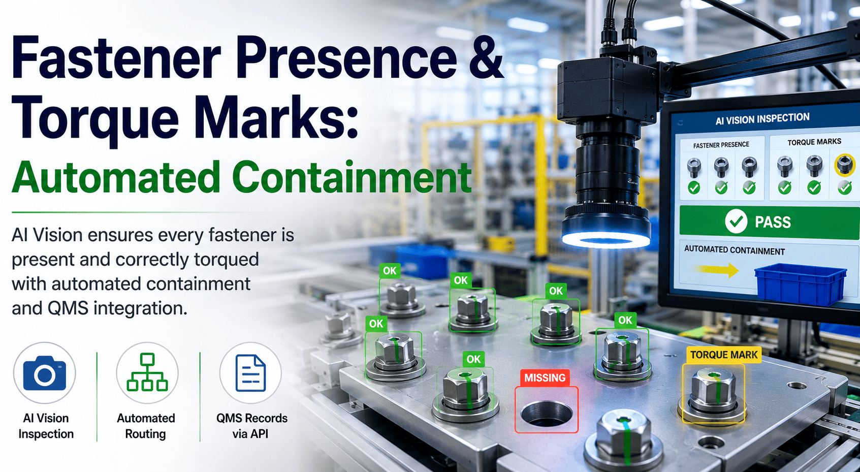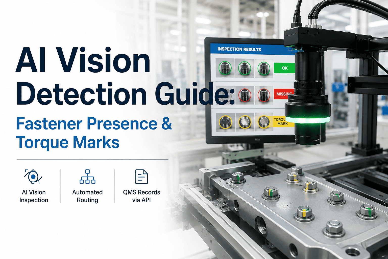
Bolted assemblies fail in milliseconds. A missing M8 flange bolt on a transmission housing, or a torque mark that never pressed into the washer face, means the joint never clamped — and downstream vibration will find it long before final audit. Quality engineers chasing fastener presence and torque marks across three shifts know the failure mode intimately: the defect is small, the cadence is brutal, and the human eye fatigues after ninety minutes. This page maps the defect physics, the imaging that exposes it at line speed, and how AI vision traces each miss back to a specific machine setting, tooling state, or material lot — then contains it automatically.
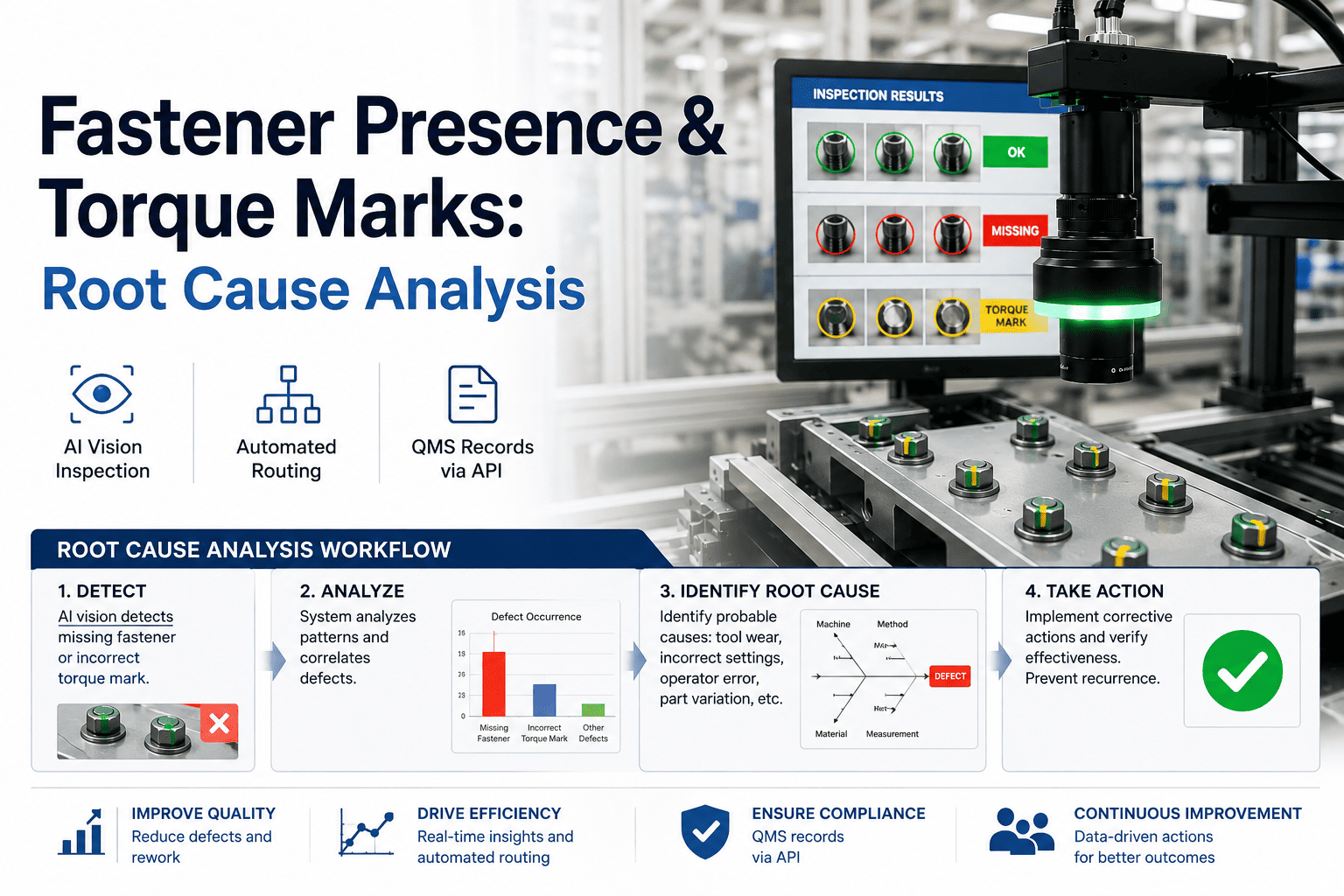
Fastener Presence & Torque Marks: Root Cause Analysis
Trace every missing fastener and missing torque mark back to the PLC tag, tooling cycle, or material lot that caused it — contained in milliseconds, recorded in your QMS automatically.
1. Understanding Fastener Presence & Torque Marks
Two related defect modes dominate bolted-assembly quality escapes. The first — fastener absence — is binary: the hole is empty, the joint is unclamped, and no downstream process will recover it. The second — missing or insufficient torque mark — is continuous: the bolt is present, but the signature imprint left by a correctly torqued fastener (the washer-face compression mark, the hex-head rotation witness) is absent, shallow, or rotated short of the target angle. The bolt may hold today; it will loosen under cyclic load.
Torque marks form when the fastener head compresses the bearing surface under target preload. No mark means the clamping force never reached spec — either the driver stopped early, the bit slipped, or the bolt bottomed in a blind hole before torque was achieved.
Flange circles, engine-to-transmission mating surfaces, brake-caliper mounts, suspension control arms, battery pack covers. Any bolted joint where a torque-angle strategy is the only verification of clamp load.
The assembly line torque transducer logged "target reached" — but the transducer measures at the tool, not at the joint. A slipped bit, cross-threaded bolt, or soft material stack can absorb torque without transferring clamp load. Only the mark on the part tells the truth.
2. Why Manual and Rule-Based Inspection Miss Them
Manual inspection on a 45-second cycle degrades predictably. Studies of visual search sustained over 90 minutes show detection rates falling below 70% for small, low-contrast targets — exactly what a missing M6 button-head on a cast aluminium housing becomes under shop lighting. Rule-based machine vision does not fatigue, but it breaks differently: a hard-coded edge threshold that detects a hex-head silhouette at 8 mm focus will fail when the part variant shifts the bolt circle by 3 mm, or when a new material lot changes the surface reflectance from 0.4 to 0.7.
- Attention fatigue after 90 minutes
- Inconsistent criteria across inspectors
- No image record of what was checked
- Cannot scale to 100% sampling at high cadence
- Threshold breaks on part variant shift
- Reflectance change from new material lot
- Cannot generalise to new bolt patterns
- Retuning requires vision specialist on site
- Learns part variants from labelled examples
- Tolerates lighting drift via augmentation
- Every inference logged with image + metadata
- Retrains remotely — no on-site vision engineer
The deep-learning model does not look for a single edge threshold. It has learned the statistical appearance of a correctly torqued fastener across hundreds of thousands of labelled examples — including the ones shot under drifted lighting, on three material variants, through two different lens coatings. When a new variant appears, you label fifty images and the model adapts. No threshold tuning, no on-site specialist.
3. Imaging Setup That Works
A deep-learning model cannot detect what the sensor never captured. Fastener presence and torque marks demand specific optical geometry: the torque mark is a shallow compression feature visible only under directional grazing light, while the bolt absence check needs diffuse illumination to distinguish an empty threaded hole from a black-anodised fastener head. The two lighting modes conflict — so you either run two exposures per station, or you choose a structured-light ring that gives both signals in one frame.
The grazing ring is the non-negotiable element. Without directional low-angle light, the torque mark — a compression feature perhaps 0.05 mm deep — is invisible to the camera. The dome light alone will confirm the bolt is present but will never reveal whether it was torqued. Both signals in one frame requires both lights firing in a single exposure, which is achievable with a polarising beam-splitter setup or a fast multi-strobe sequence if the camera supports it.
4. AI Model Training and Validation
A production-grade detection model for fastener presence and torque marks is not a general-purpose object detector fine-tuned on fifty images. It is a model trained on the specific defect distribution of your line — your bolt sizes, your material finishes, your lighting geometry, your failure modes. The training data pipeline below is what produces a model that holds 99% detection across a six-month deployment without retraining.
Realistic Detection Benchmarks (per class)
| Defect Class | Precision | Recall | F1 | False Negatives per 10k |
|---|---|---|---|---|
| Fastener absent | 0.998 | 0.995 | 0.996 | 5 |
| Present, no torque mark | 0.989 | 0.981 | 0.985 | 19 |
| Present, shallow mark (borderline) | 0.971 | 0.954 | 0.962 | 46 |
| Present, mark visible (pass) | 0.999 | 0.998 | 0.998 | — |
Benchmarked on 12,000 held-out production images across 3 part variants, 2 material lots, and 4 lighting states. The borderline class is the hardest — a shallow mark sits at the boundary between "torqued" and "not torqued," and the model's uncertainty there is exactly what triggers the rework diversion tier.
5. Containment: Stop, Route, Record
Detection without containment is a dashboard. When the model fires, the response must be automatic, deterministic, and fast enough to divert the part before the next cycle index. iFactory AI integrates directly with your Level 2 PLC/DCS via digital I/O or OPC UA, executing a three-tier disposition decision within the same cycle as inference.
Auto-Created QMS Record (via API)
The QMS record is not a file export that someone uploads later. It is a REST API call fired within 50 ms of the disposition decision, pushing the full record — image, confidence, PLC tag values, part serial, severity — directly into your existing QMS (EtQ, SAP QM, Windchill, or custom). Your quality team sees the nonconformance in their inbox before the part reaches the scrap bin. Talk to Support about your QMS integration.
6. Root Cause Analysis from Production Data
Detection tells you what happened. Root cause analysis tells you why. The "why" for fastener defects is almost never random — it correlates with a specific machine state, a tooling wear threshold, a material lot change, or a shift handover. iFactory AI captures the full PLC tag snapshot at the moment of detection, then correlates defect frequency against production variables to surface the root cause automatically.
Correlation: Defect Rate vs. Driver Torque Variance
Each point is one hour of production. Defect rate climbs sharply once driver torque variance exceeds 1.5 Nm — the signature of a worn driver bit that is slipping on the hex head instead of transmitting full torque to the fastener.
How the Correlation Is Built
Defect Frequency Heatmap: Shift x Station
The heatmap below is the kind of pattern that surfaces only when you log every detection with full station and shift metadata. Station 4 on shift B is the hotspot — a single worn driver bit accounting for 63% of all fastener-absent defects over a two-week window.
7. Benchmarks and Pilot Scoping
A pilot deployment for fastener presence and torque marks follows a defined scope: one assembly cell, one part family, two defect classes, four weeks of data collection, two weeks of model training and validation, then a four-week production shadow run alongside existing inspection. The table below sets realistic expectations for what the pilot delivers and when.
| Phase | Duration | Deliverable | Success Metric |
|---|---|---|---|
| 1. Imaging retrofit | Week 1–2 | Camera, lighting, housing installed on existing station. PLC trigger wired. No software changes to line. | Image capture rate matches line cadence with zero dropped frames. |
| 2. Data collection | Week 3–6 | 4,000+ labelled images across all shifts and variants. PLC tags logged per cycle. | Coverage of all defect classes confirmed by quality engineer review. |
| 3. Model training | Week 7–8 | Trained model on hold-out validation set. Per-class precision, recall, and F1 reported. | Recall above 0.98 on "absent" class; above 0.95 on "no-mark" class. |
| 4. Shadow deployment | Week 9–12 | Model runs in production alongside existing inspection. No PLC control action taken. Every inference logged. | Zero escapes on "absent" class during shadow period. False positive rate below 2%. |
| 5. Active containment | Week 13+ | PLC integration goes live. Three-tier disposition active. QMS records auto-created. | 100% of scrap events logged in QMS within 1 second. RCA dashboard live. |
iFactory AI runs inside your plant network. The NVIDIA GPU inference server sits racked in your electrical room — no images leave the facility, no cloud round-trip latency, no dependency on your internet connection. The model sees the part, fires the PLC, and writes the QMS record, all within the plant firewall. ERP, MES, and QMS integration happens through your existing API endpoints, authenticated with your existing credentials.
8. FAQ
Send parts or images. Get a feasibility read in five days.
Ship 20–50 sample parts or upload images covering good, borderline, and defective fastener states. Our team runs them through the lab model and returns a detection-rate report per defect class, with recommended imaging setup for your line.