On a high-volume brake-caliper line, a single missing torque-mark signature on a caliper bolt can mean the joint was never tightened to spec — and the bolt will back out under vibration. Manual inspectors catch maybe 80% of these on a good shift, far fewer on hour ten. The hard part is not seeing the defect once; it is sustaining attention across 4,000 assemblies per shift while part variants and ambient lighting drift. Deep-learning vision trained on bolted-assembly defects holds detection rates manual inspection cannot, and — this is the part that matters to a process engineer — it can fire a containment signal to your PLC in under 50 milliseconds, routing the assembly to rework or scrap before the next station even sees it. Book a demo to see it on your parts, or read on for the imaging, training, and containment architecture.
Automated containment for bolted-assembly defects — detection to disposition in milliseconds
On-prem GPU inference retrofitted to your existing line. Good parts proceed, borderline parts divert to rework, hard failures drop to scrap — with QMS records written automatically via API.
Understanding fastener presence & torque marks
Two related defect classes, same joint. Fastener presence is binary — the bolt is there or it is not. Torque marks are the witness signature left by the tightening tool: a paint dab, a scribe line, or a deformation pattern that proves the tool engaged and reached target torque. Both must be verified on every bolt of every assembly.
- Bolt omitted during assembly
- Bolt dropped, not seated
- Wrong bolt variant installed
- Tool engaged but torque not reached
- Operator skipped tightening step
- Mark washed off or misapplied
Where these defects occur on a typical bolted assembly
Why manual and rule-based inspection miss them
Rule-based vision systems fail on bolted assemblies because the defect is not a geometric deviation — it is the absence of a feature that varies in position, angle, and appearance. A missing torque-mark dab looks different on every part variant. Manual inspection fails for a simpler reason: sustained vigilance is not a human trait.
Three ways rule-based vision breaks on torque marks
A rule-based system looks for a dab within a pixel window. Rotate the part 3 degrees on the fixture and the dab leaves the window — false reject cascade begins.
A blob-detection threshold tuned at 9 AM fails by 2 PM when ambient light shifts. Operators learn to "accept all" to keep the line running.
Rule-based vision detects features that are present. It has no native way to reason about a feature that should be there but is not — the core of the torque-mark problem.
Imaging setup that works
Detection quality is bounded by image quality. The goal is to make the torque-mark signature — whether a paint dab, scribe line, or deformation — visible at line speed without motion blur, and to do it consistently across part variants and shift lighting.
Lighting strategy by mark type
Bars show relative effectiveness of each lighting mode for each mark type. Deep purple = strong signal, light = weak. Most lines need two lighting channels to cover mixed mark types on the same assembly.
AI model training and validation
A detection model is only as good as the data it was trained on. For fastener presence and torque marks, the training set must cover the full range of part variants, mark types, lighting conditions, and — critically — the failure modes. A model trained only on good parts will never learn what a missing torque mark looks like.
Data composition by class
Minimum viable training set for a single assembly family. Augmentation (rotation, brightness, blur) expands effective set 5–8x without collecting new physical samples.
Validation confusion matrix
The 2.1% false-negative rate is the number that matters for safety-critical joints. iFactory tunes the decision threshold to push FN below 0.5% at the cost of a higher FP rate — false rejects go to manual review, false escapes go to the customer.
Labeling strategy — what to annotate and why
Containment: stop, route, record
Detection without containment is just a dashboard. The value is in what happens next: the moment the model flags a defect, a containment signal fires to the Level 2 PLC/DCS, and the assembly is physically routed — good parts proceed, borderline parts divert to rework, hard failures drop to scrap. All of this happens in milliseconds, before the next station touches the part.
Proceeds to next station. QMS record logged as pass with image retained for traceability.
Diverts to rework lane. Operator reviews image on HMI, re-tightens or re-marks, re-enters inspection.
Drops to scrap chute. Full image set, PLC tags, and severity score written to QMS via API for RCA.
QMS record — auto-created per defect
| Field | Source | Example value |
|---|---|---|
| Assembly serial | PLC tag at capture | CAL-2024-08471 |
| Defect class | AI model output | TORQUE_MARK_ABSENT |
| Bolt position | Model localization | Pos 3 of 6 (flange) |
| Confidence score | Model output | 0.31 |
| Disposition | Containment logic | SCRAP |
| Capture image | Camera frame | img_08471_003.png |
| PLC tag snapshot | Level 2 at defect time | torque_set=45N·m, actual=0N·m |
| Timestamp | System clock | 2024-11-14T14:23:07.412Z |
| Shift / Operator | MES integration | Shift 2 / Line A |
Every field is written via REST API to your existing QMS ( SAP DMS, Windchill, Plex, or custom ). No manual data entry, no clipboard, no end-of-shift reconciliation. The record exists the moment the part hits the scrap chute. Talk to support about your QMS integration.
Root cause analysis from production data
When defects cluster — say, torque marks missing on position 3 across 40 consecutive assemblies — the question is not "did the model catch them?" (it did) but "what changed?" iFactory captures PLC tags at defect time, so you can correlate defect bursts with upstream process variables without manual data hunting.
Defect burst — position 3, shift 2, Nov 14
Correlated PLC tags during burst
Torque tool 3 stopped cycling (actual torque = 0 N·m) while the controller still reported "target reached." The AI vision system caught the missing torque mark on every assembly the tool failed to tighten — 47 consecutive defects contained, zero escapes to customer.
Benchmarks and pilot scoping
Realistic detection benchmarks for fastener presence and torque marks, grounded in production deployments across automotive, aerospace, and industrial equipment assembly lines. Numbers below reflect steady-state performance after model tuning — not first-day results.
Pilot scoping — what to send, what you get back
Send us parts or images and get a feasibility read in one week. Book a demo to start the conversation.
Frequently asked questions
Can the model handle new part variants without retraining from scratch?
Yes. Transfer learning from an existing bolted-assembly model typically requires 50–150 new labeled images per variant to reach production detection rates. The base model already understands bolt positions, mark types, and lighting variation — new variants are incremental, not a restart.
How does the system handle lighting drift across shifts?
Two layers: first, controlled lighting (dome + coaxial) minimizes ambient influence at capture time. Second, the model is trained on augmented images spanning brightness ranges wider than any real shift drift. If drift exceeds the training distribution, the system flags a "model confidence degradation" alert rather than silently degrading.
What PLC and DCS protocols are supported for containment signals?
Modbus TCP, EtherNet/IP, PROFINET, and OPC UA are supported natively. The containment signal is a simple discrete tag write — disposition code and assembly serial — fired in under 50ms from inference completion. No custom middleware required.
Does the system run inside our plant network, or does it need cloud?
It runs entirely inside your plant network. GPU inference is on-prem on an NVIDIA AI server racked in your facility. No images leave the plant. The only external connection is the optional QMS API if your QMS is cloud-hosted — and even then, only metadata is transmitted, not raw images.
How are borderline parts handled differently from clear defects?
The model outputs a continuous confidence score. Parts scoring between 0.50 and 0.92 are routed to a rework lane where an operator reviews the image on an HMI and makes the final call. Parts below 0.50 drop to scrap automatically. The thresholds are configurable per assembly family and per bolt position.
What happens to the images after they are captured?
Every image is retained for the traceability period your QMS requires (typically 1–7 years). Good-part images are stored at reduced resolution; defect images are stored at full resolution with annotations. Storage is local on the GPU server, with optional archival to your existing NAS or SAN.
Send us your parts. Get a feasibility read in one week.
Send 50–200 assemblies with known good and defective samples. We will label, train a baseline model, and report expected detection rates, false-negative rates, and imaging requirements specific to your bolted assemblies — before you commit to a pilot.