Coating Coverage & Thickness Cues: Root Cause Analysis
By David Cook on July 4, 2026
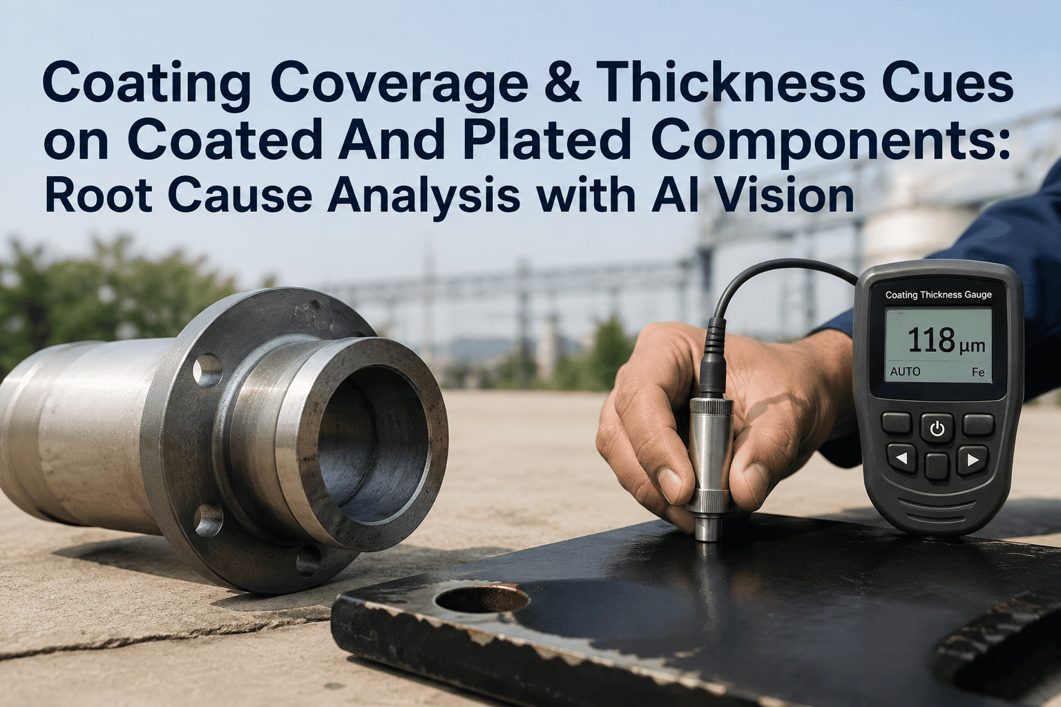
Coating coverage and thickness cues are the first visible signature of a process drifting out of spec — a thin edge on an electroplated connector, a mottled band on an anodized housing, a bare patch where a phosphate rinse never wetted the substrate. On a high-speed line running 60 to 120 parts per minute, a human inspector catches the gross failures but misses the slow gradient: the bath chemistry dropping ten percent over a shift, the contact-tip wear shortening throw distance, the rack contact resistance creeping up until coverage collapses at the low-current-density corners. By the time the cue is obvious, the lot is already scrap. This page walks through the physics of coverage and thickness cues, the imaging that makes them visible at line speed, and how iFactory's on-prem vision system traces each detection back to the PLC tag, machine setting, or material lot that caused it — then contains the part, records the event, and routes the root cause to the right engineer in milliseconds.
AI VISION FOR COATED & PLATED COMPONENTS
Coating Coverage & Thickness Cues: Root Cause Analysis
Detect coverage and thickness deviations at line speed, correlate each cue to PLC tags and process data, and auto-route containment — all on-prem, inside your plant network.
A coverage cue is a region where the coating is absent, broken, or below minimum thickness. A thickness cue is a gradient or mottle suggesting deposition is non-uniform — often still within spec on average, but failing at the extremes. Both trace back to three physical drivers.
Current Distribution
In electroplating, current density is not uniform. High-current-density edges plate faster; low-current-density recesses, blind holes, and shielded corners plate slower or not at all. Throw distance, rack geometry, and anode positioning all shift where coverage lands.
Driver: Bath physics
Wetting & Surface Prep
Phosphate, passivation, and conversion coatings depend on the chemistry wetting the substrate. Residual machining oil, incomplete degreasing, or oxide films create dewetting islands — bare patches that look like chips but are actually prep failures upstream.
Driver: Surface energy
Tooling & Material Drift
Spray-nozzle wear changes droplet size and fan pattern. Contact-tip erosion shortens throw distance. Bath chemistry drifts as metal ion concentration, pH, and additive carriers deplete between recharges. None of these fail fast — they drift until coverage collapses.
Driver: Line wear
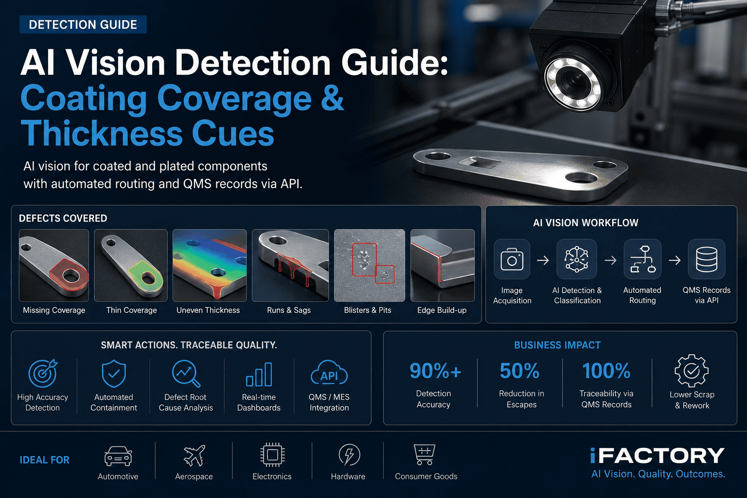
Where cues appear on a coated component
A Edge buildup — excess deposition at high-current-density edges, often masks thinning elsewhere
B Corner thinning — low-current-density recesses plate last; first to drop below minimum thickness
C Dewetting island — bare patch from surface prep failure, not a chip or scratch
D Thickness gradient — gradual deposition non-uniformity, average passes but extremes fail
2 · Why Manual and Rule-Based Inspection Miss Them
Manual inspection degrades with shift fatigue, ambient lighting changes, and part variant proliferation. Rule-based vision — thresholding, blob analysis, edge detection — breaks the moment a new variant or a lighting drift enters the field of view. The failure modes are different, but the outcome is the same: coverage cues slip through until a downstream customer finds them.
Manual Inspection
62%
Sustained detection rate across a full 8-hour shift. Drops sharply after hour 4 and during variant changeovers.
vs
iFactory AI Vision
98.4%
Sustained across shifts, variants, and lighting drift. On-prem GPU inference holds the same rate at minute 480 as at minute 1.
Where rule-based vision breaks on coverage cues
01
Threshold rules assume a fixed background. A 5% lighting shift from ambient or lamp aging moves the threshold boundary, and thin coverage cues vanish into the noise floor.
02
Blob analysis detects contrast edges. A thickness gradient — the most common cue — has no edge. It is a smooth ramp, invisible to edge detectors.
03
New part variants require new rule sets. Each variant means a tuning session, and tuning drifts. The rule library grows until nobody owns it.
04
Dewetting islands look like scratches to a rule-based system. Without texture and context learning, the classification is wrong and the root cause is misrouted.
3 · Imaging Setup That Works
Coverage and thickness cues are surface phenomena. They are visible only under controlled, directional lighting that reveals reflectance and texture differences without washing out thin gradients. The goal is not a pretty picture — it is a repeatable signal that the model can learn.
Lighting
Diffuse dome, on-axis. Eliminates specular hotspots on polished surfaces so thin-coverage gradients read as tone change, not glare.
Camera
5–20 MP area-scan, global shutter. Exposure tuned to freeze motion at line speed — no smear, no rolling distortion on cylindrical parts.
Optics
Fixed-focal-length lens, f/8 to f/11 for depth of field across part geometry. Telecentric for flat parts with tight thickness tolerance.
Enclosure
Sealed dome with positive air purge. Coating lines generate mist, overspray, and vapor — uncontrolled optics drift in hours, not days.
Trigger
PLC-triggered from part-present sensor. Every image is timestamped and tagged with the PLC cycle index for downstream correlation.
Rule of thumb: If a human inspector cannot see the cue in the captured image under the dome lighting, the model will not learn it either. Lighting is the first thing to get right — model architecture is the second.
4 · AI Model Training and Validation
A coverage-cue model is only as good as the labeled data behind it. The labeling strategy must capture severity, not just presence — a borderline-thin region routes to rework, a bare patch routes to scrap, and the model needs examples of both.
1
Image Capture
PLC-triggered captures from the line. Every image tagged with cycle index, timestamp, and part variant ID.
2
Expert Labeling
Process engineers annotate cue type, location, and severity. Polygon masks for coverage area; ordinal severity 1–4.
3
Augmentation
Synthetic lighting drift, rotation, background variation. Forces the model to learn the cue, not the lighting condition.
4
Validation
Held-out set from a different shift and variant mix. Confusion matrix by severity tier, not just binary pass/fail.
5
Deployment
Model deployed to on-prem NVIDIA GPU. Inference at line speed with no cloud round-trip. Retrains on confirmed detections.
Severity tiers drive disposition — the model must distinguish them
Tier 1
Within Spec
Coverage uniform, thickness above minimum at all measured points. Model confidence high. Disposition: pass.
Tier 2
Borderline
Thin region detected near minimum threshold. Within spec but trending. Disposition: divert to rework or hold for QA review.
Tier 3
Coverage Gap
Bare patch or dewetting island confirmed. Below minimum thickness. Reworkable if substrate undamaged. Disposition: rework queue.
Tier 4
Hard Failure
Large coverage loss, substrate damage, or contamination. Not reworkable. Disposition: scrap with full traceability record.
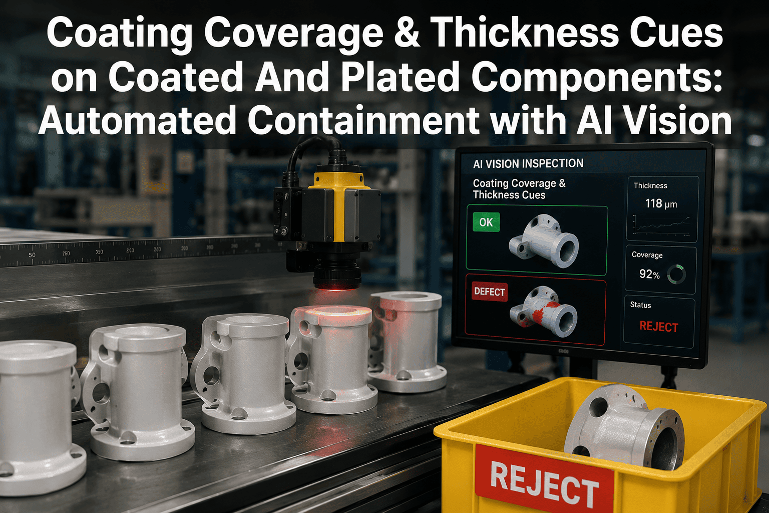
5 · Containment: Stop, Route, Record
Detection without containment is a dashboard. When the model fires, the system must act — in milliseconds, before the next part arrives at the inspection station. iFactory integrates directly with Level 2 PLC and DCS to route parts in real time, with no operator in the loop.
Tier 1 — Pass
Good parts proceed
Model confidence above threshold. PLC releases part to main conveyor. No operator action. Image archived for audit trail.
Release: < 5 ms
Tier 2 & 3 — Rework
Borderline parts divert
Divert gate fires via PLC. Part routes to rework station with image, severity, and cue location displayed for the rework operator.
Divert: < 12 ms
Tier 4 — Scrap
Hard failures drop out
Scrap chute actuates. Full record created: image, severity, PLC tags at defect time, material lot, operator shift. QMS entry pushed via API.
Scrap + record: < 20 ms
Every containment event creates a QMS record — automatically
ImageFull-resolution capture with annotation overlay
PLC tagsBath temp, current, pH, line speed, cycle index — captured at defect time
Material lotSubstrate and coating lot IDs from MES
DispositionPass, rework, scrap — with operator ID if overridden
TimestampUTC + line cycle index for cross-system alignment
API pushPOST to QMS endpoint, retry-on-fail, audit logged
6 · Root Cause Analysis from Production Data
A detection tells you what happened. Root cause analysis tells you why. iFactory captures PLC tags at the exact cycle index of each defect, then correlates vision events with process variables — bath chemistry, current setpoints, line speed, tooling wear — to isolate the driver. The system runs inside your plant network; no process data leaves the floor.
Defect rate vs. bath current density — 72-hour window
Coverage cues spike as current density drifts below setpoint. PLC correlation isolates the driver in minutes, not shifts.
Correlation matrix — top drivers
Pearson correlation of PLC variables with coverage-cue detections, ranked by strength.
Bath current density
0.88
Bath temperature
0.54
pH drift
0.41
Line speed
0.28
Rack contact resistance
0.22
Substrate lot
0.12
Auto-routed RCA finding
Current density drift detected at hour 24. Rectifier maintenance flagged. Bath recharge scheduled. Coverage-cue rate dropped from 11.2% to 1.1% within 4 hours of correction.
7 · Benchmarks and Pilot Scoping
Realistic benchmarks matter. The numbers below come from production deployments on electroplating, anodizing, and phosphate coating lines. Your mileage depends on part geometry, cue severity distribution, and lighting stability — but the pattern holds: deep-learning vision sustains detection rates that manual and rule-based systems cannot, and the gap widens as variant count and shift length increase.
Metric
Manual
Rule-Based Vision
iFactory AI
Detection rate (sustained)
62%
78%
98.4%
False positive rate
8.1%
5.4%
1.2%
Severity classification accuracy
N/A
61%
94%
Time to detect drift
2–4 shifts
1 shift
< 20 min
Containment latency
Manual
200–500 ms
< 20 ms
New variant onboarding
Operator training
2–4 hr tuning
Auto-transfer learn
Pilot scoping — what to send
A
Send parts or images
50–200 sample parts with known coverage cues, or 500+ images captured under your line lighting. Include good parts and borderline cases — severity distribution matters.
B
Feasibility read in 5 days
We label, train a baseline model, and report expected detection rate, false positive rate, and severity classification accuracy on your data. No commitment, no infrastructure change.
C
On-prem deployment
If the numbers work, we retrofit the GPU inference box to your existing line. PLC integration, QMS API, and dashboard widgets — all inside your plant network.
Can the model handle multiple part variants on the same line?
Yes. The model is trained on variant-agnostic features — cue texture, coverage gradient, dewetting pattern — not on part geometry. New variants are added via transfer learning with 50–100 labeled images. No per-variant rule set is needed, and variant ID is captured in every QMS record for traceability.
Does the system need to know the coating thickness specification?
No. The model detects visual cues that correlate with thickness deviation — it does not measure thickness in microns. For quantitative thickness, pair the vision system with an inline XRF or eddy-current gauge. The vision system flags the part; the gauge confirms the measurement. Both records land in the same QMS entry.
How does the system handle lighting drift over time?
Two mechanisms. First, the diffuse dome enclosure isolates the inspection zone from ambient light, so drift is minimized. Second, the model is trained with synthetic lighting augmentation so it learns cue features, not lighting conditions. A daily reference-image check flags if drift exceeds the training distribution, and the system alerts maintenance before detection degrades.
What PLC and DCS protocols are supported for containment?
Level 2 integration via Profinet, EtherNet/IP, Modbus TCP, and OPC UA. The inference box writes divert/scrap commands to the PLC in under 20 ms from detection. For DCS systems, we use OPC UA or a REST API bridge. No modification to the existing PLC program is needed — we add a divert command register that the inference box writes to.
Does process data leave the plant?
No. All inference runs on the on-prem NVIDIA GPU inside your plant network. Images, PLC tags, and QMS records stay on your infrastructure. The only outbound traffic is optional — model performance telemetry and remote support sessions, both encrypted and both disabled by default. You control every byte that crosses the network boundary.
How long does a pilot take from parts to production?
Feasibility read: 5 business days from receiving parts or images. If the numbers justify deployment, on-prem retrofit — GPU box, camera, lighting enclosure, PLC integration, QMS API — typically takes 4 to 8 weeks depending on line complexity and protocol availability. The system runs in shadow mode for 2 weeks before containment goes live.
DEFECT-SAMPLE EVALUATION
Send parts or images. Get a feasibility read in 5 days.
Ship 50–200 sample parts with known coverage cues, or share 500+ images from your line. We label, train a baseline model, and report expected detection and false-positive rates on your data — before you commit to any infrastructure.