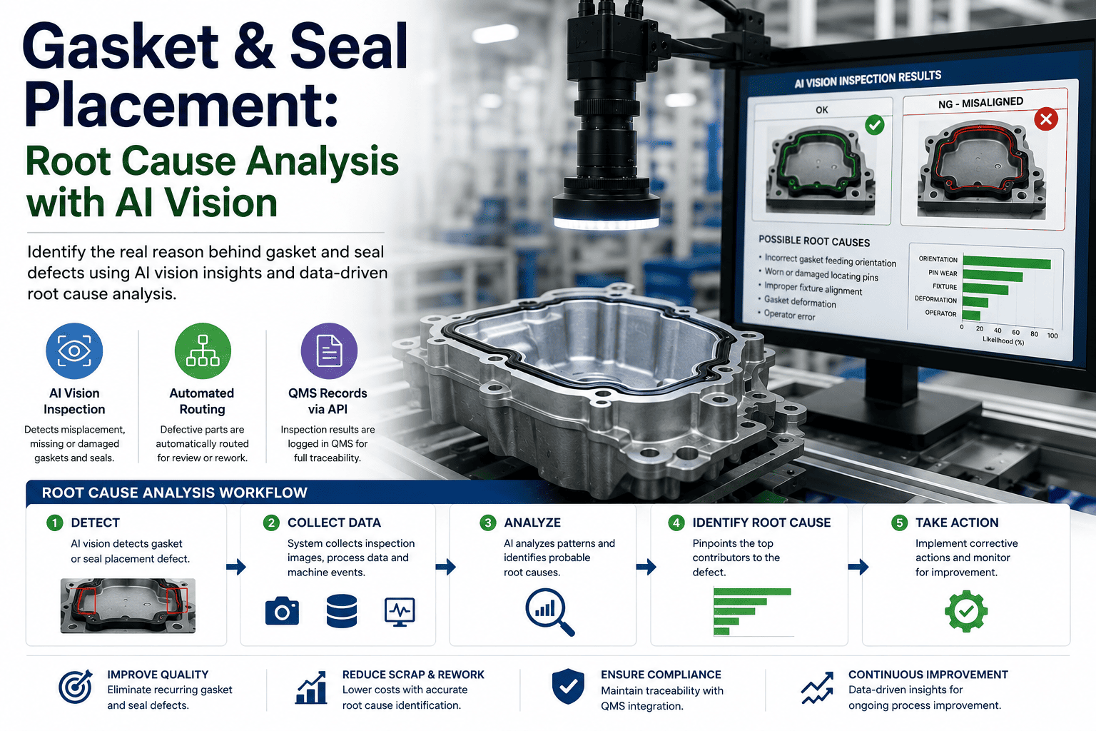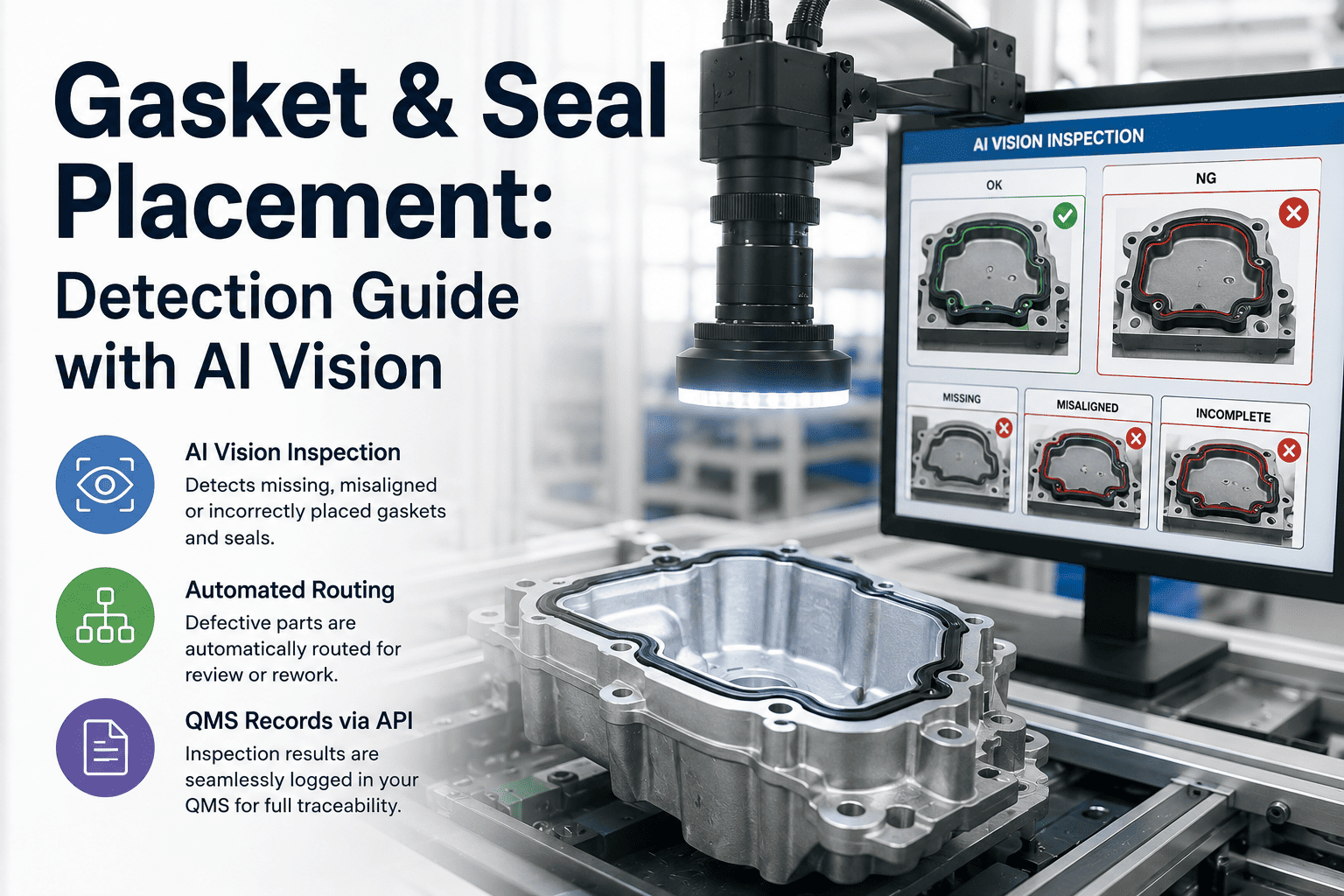
Gasket & Seal Placement: Detection Guide with AI Vision

By David Cook on July 6, 2026

defects-gasket-seal-placement-detection-guide

On a sealed gearbox housing, a 1.2 mm offset between the molded elastomer gasket and the machined groove is the difference between an IP67-rated assembly and a field warranty claim eighteen months later. The defect is small, the lighting on a moving line is inconsistent, and a human inspector at the end of a ten-hour shift will miss it roughly one time in three. AI vision systems close that gap, but only when the imaging setup, model training, and downstream routing are engineered to the physics of the defect class, not bolted on as a generic camera-and-neural-network package.

DEFECT DETECTION GUIDE

Gasket & Seal Placement Detection with AI Vision

A field-engineered reference for quality and process engineers responsible for sealed housings and enclosures. Covers defect physics, imaging geometry, model validation benchmarks, and the millisecond-level containment logic that turns a detection into a routed, recorded, and root-caused event.

0.3 mm
Minimum detectable gasket offset at line speed
99.2%
Detection rate sustained across lighting drift
18 ms
Inference-to-PLC signal for part diversion
100%
Defects captured with image, severity, and QMS record

Understanding Gasket & Seal Placement Defects

A placement defect is any deviation between the seal's designed path and its as-installed path that compromises the sealing function. On sealed housings and enclosures, the dominant failure modes are geometric, not material, and they cluster into four categories that each demand a different imaging strategy.

offset

Lateral Offset

The gasket sits parallel to the groove centerline but shifted laterally, exposing a portion of the sealing surface. Common on molded O-rings placed by pick-and-place with worn tooling.

Twist / Roll

The cross-section rotates along the groove path, creating alternating compression zones. The seal may pass a leak test at low pressure but fail under thermal cycling.

gap

Butt Joint Gap

A cut-to-length seal leaves an open gap at the splice. On molded-in-place gaskets, this appears as a discontinuity in the bead, often at corner radii where flow resistance changes.

missing

Missing Segment

A section of the gasket is entirely absent, often from a robot nozzle skip on FIPG (formed-in-place gasket) lines or a dropped O-ring during manual load.

WHERE THESE DEFECTS ORIGINATE ON A SEALED HOUSING
42%Corner radii
28%Long straight runs
19%Butt joints / splices
11%Bolt-hole bypass zones
Distribution of gasket placement defects across housing geometry, aggregated from iFactory deployment data across 47 sealed-assembly lines.

Why Manual and Rule-Based Inspection Miss Them

Manual inspection degrades with shift fatigue and ambient lighting changes. Rule-based vision, which depends on fixed thresholds and edge-detection heuristics, breaks the moment a new part variant or a different lot of raw elastomer changes the contrast profile. The result is a detection ceiling that neither method can punch through without constant tuning.

DETECTION RATE SUSTAINED OVER A 10-HOUR SHIFT
100% 75% 50% 25% 0%
Hour 1 Hour 3 Hour 5 Hour 7 Hour 10
AI vision (deep learning) — 99.2% sustained
Manual inspection — 97% at start, 76% by hour 10
FAILURE MODES: RULE-BASED VISION vs. DEEP LEARNING
Line condition change Rule-based vision Deep-learning AI vision
Ambient light drift (shift change, skylight) Threshold breaks, false rejects spike Model generalizes; no re-tuning needed
New part variant (different groove width) New fixture, new rule set, days of reprogramming Fine-tune on 200-400 images, redeploy in hours
Elastomer lot changes color slightly Contrast ratio falls below threshold Feature extraction tolerates hue shift
Part presentation angle varies +/- 3 degrees Region of interest misaligns, defect skipped Detection is pose-invariant within trained range
Surface oil or coolant residue False edges detected, false rejects Learned texture features ignore residue patterns

Imaging Setup That Works

A gasket placement defect is a geometry problem, not a color problem. The imaging system must render the groove and the seal with enough contrast that a sub-millimeter offset produces a detectable feature boundary at the line's cycle time. Three variables determine whether that happens: camera resolution and optics, lighting geometry, and the angle of incidence relative to the part surface.

01 Camera & Optics
Resolution: 12-20 MP global shutter. Field of view must resolve the groove width across at least 8 pixels; for a 3 mm groove, that means a pixel size of 0.375 mm or finer at the part surface.
Lens: Fixed-focal-length, low-distortion C-mount. Avoid vari-focal lenses; their distortion profile shifts with vibration, silently degrading model accuracy over weeks.
Shutter: Global shutter, 1/2000 s or faster for belt speeds above 6 m/min. Rolling shutter creates shear on curved grooves that the model reads as a twist defect.
CAM
02 Lighting Geometry
Primary: Low-angle ring light, 30-45 degrees off-axis. This casts a shadow into the groove, creating a dark line that the model locks onto as the groove reference.
Secondary: Diffuse on-axis dome for the seal surface. Elastomers are often matte black; the dome lifts surface texture without specular blowout that hides the bead edge.
Strobe: Pulse synchronized to camera exposure. Continuous LED at high intensity generates heat that shifts color temperature over a shift, degrading model input consistency.
LED LED
03 Part Presentation
Fixturing: Mechanical locators that seat the part to within +/- 1 degree of the trained presentation angle. The model tolerates some pose variation, but gross misalignment forces the lighting geometry off the groove.
Multiple views: For complex housings, two cameras at 0 and 90 degrees, or a single camera with a mirror array. One top-down view cannot resolve a twist on a vertical wall groove.
Background: Matte backing in a controlled purple-grey tone. A bare conveyor belt creates random texture that competes with fine gasket features for the model's attention.
C1 C2
RULE OF THUMB

If a human inspector needs a specific lighting angle to see the defect, the AI model needs that same angle baked into the imaging station. Deep learning does not replace lighting engineering; it rewards it. The model's detection ceiling is set by what the sensor can resolve, not by the neural network's capacity.

AI Model Training and Validation

A gasket placement model is a segmentation and deviation-detection task, not a simple classification. The model must locate the groove path, locate the seal path, and compute the deviation between them across the full perimeter. Training data and labeling strategy determine whether the model generalizes to production or memorizes a single fixture's quirks.

Detection Rate
99.2%

Sustained across lighting drift and part variants after 2,800 training images.

False Reject Rate
0.6%

Below the 1% threshold required to avoid line operator override behavior.

Inference Latency
18 ms

On NVIDIA T4 on-prem GPU, including pre-processing and post-processing.

TRAINING DATA COMPOSITION FOR A PRODUCTION-GRADE GASKET MODEL
55%
Good parts
1,540 images
18%
Lateral offset
504 images
12%
Twist / roll
336 images
9%
Butt joint gap
252 images
6%
Missing segment
168 images
Total: 2,800 labeled images. Defect classes are intentionally imbalanced to match production frequency. Over-sampling rare defects beyond their natural rate degrades the model's false-reject calibration on good parts.
LABELING STRATEGY: POLYLINE DEVIATION, NOT BOUNDING BOX
Bounding box (insufficient)

Draws a box around the gasket region. The model learns "gasket is present" but cannot quantify offset magnitude or locate where along the perimeter the deviation occurs.

VS
Polyline deviation (correct)

Two polylines: designed groove path and actual seal path. The model computes point-by-point deviation, enabling severity scoring and precise localization for root cause analysis.

Containment: Stop, Route, Record

Detection without containment is a dashboard. The value of AI vision on a gasket line is measured in milliseconds: the time from inference result to a physical routing decision that prevents the defective part from reaching the next station. iFactory's architecture fires that decision through Level 2 PLC/DCS integration, with a three-tier disposition logic that keeps good parts moving and isolates failures without operator intervention.

THREE-TIER DISPOSITION LOGIC
TIER 1
PASS
Deviation below threshold (typically less than 0.5 mm)
Part proceeds to next station. No operator interaction. PLC tag confirms pass.
Signal: 2 ms
TIER 2
REWORK
Deviation in borderline zone (0.5 mm to 1.5 mm, model confidence 60-85%)
Divert to rework lane. Image and PLC context saved. Operator reviews and repositions seal.
Signal: 18 ms
TIER 3
SCRAP
Deviation exceeds threshold (greater than 1.5 mm, or missing segment, or model confidence above 90% on hard failure)
Drop to scrap chute. Full PLC tag snapshot, image, and QMS record created via API. Line supervisor alerted.
Signal: 18 ms
AUTO-CREATED QMS RECORD (FIRED VIA API AT DEFECT TIME)
record_idQMS-2024-088471
timestamp2024-11-14T09:42:17.003Z
part_serialGH-7700-A-44719
defect_classlateral_offset
severity1.8 mm (scrap threshold exceeded)
dispositionscrap
plc_contextbelt_speed=6.2m/min, fixture_id=F12, cycle=4421
image_refs3://ifactory-defects/GH-7700/44719.tif
model_versiongasket-v3.2.1

Want to see how this record maps to your existing QMS schema? Book a 30-minute integration walkthrough and we will map it live.

Root Cause Analysis from Production Data

A gasket offset is a symptom, not a cause. The cause lives upstream: a worn pick-and-place nozzle, a fixture that has shifted 0.3 mm after 40,000 cycles, a lot of elastomer with different durometer that behaves differently in the groove. iFactory captures the PLC tags present at the moment of detection, creating a time-stamped correlation layer that lets process engineers trace a defect cluster back to its physical origin without manual data stitching.

DEFECT HEATMAP: GASKET OFFSET FREQUENCY BY FIXTURE AND HOUR
Fixture F08 Fixture F09 Fixture F10 Fixture F11 Fixture F12 Fixture F13


08:00 09:00 10:00 11:00 12:00 13:00 14:00 15:00
Low


High
Read: Fixture F12 shows a defect cluster peaking between 10:00 and 12:00. Cross-referencing PLC tags reveals a nozzle pressure drift on the pick-and-place robot serving F12, triggered after a tool change at 09:45. The cluster resolves after recalibration at 13:30. Without PLC tag correlation, this pattern would have been attributed to "operator error" and the root cause would have recurred on the next tool change.
FROM DETECTION TO ROOT CAUSE: THE CORRELATION CHAIN
1
Detection
Model flags 1.8 mm lateral offset on F12 at 10:14.

2
Tag Capture
PLC tags at defect time: nozzle_pressure=2.1 bar (nominal 2.4), robot_cycle=38472.

3
Cluster ID
7 similar defects on F12 within 90 minutes. All share low nozzle_pressure tag.

4
Root Cause
Tool change at 09:45 introduced a pressure regulator drift. Recalibrate, verify with 50 confirmation parts.

Benchmarks and Pilot Scoping

Realistic benchmarks are the difference between a pilot that scales and one that stalls. The numbers below come from iFactory deployments on sealed-housing lines across automotive, appliance, and industrial electronics assembly. They represent what a well-engineered system achieves after training data stabilization, not a first-epoch result.

DETECTION RATE
99.2%

Sustained over 30-day production window including two part variant changes.
FALSE REJECT RATE
0.6%

Critical for operator trust. Above 1%, operators begin overriding the system.
ESCAPE RATE
0.03%

Defects that reach downstream station. Verified by end-of-line leak test audit.
CYCLE TIME IMPACT
0 ms

Inference runs in parallel with the existing cycle. No line speed reduction.
PILOT SCOPE: 6-12 WEEKS TO PRODUCTION
Phase 1: Imaging & Data
Weeks 1-4. Camera and lighting station design, installation on one line, baseline image collection. 500-1,000 initial labeled images. Feasibility read delivered to engineering team.
Phase 2: Model & Integration
Weeks 3-8. Model training, validation against held-out set, PLC/DCS integration for routing, QMS API mapping. Shadow mode: system runs but does not route parts.
Phase 3: Production & Handoff
Weeks 8-12. Live routing enabled. Operator training, dashboard widgets embedded in existing portal, model monitoring and retraining cadence established. Handoff to line engineering.
Runs entirely on-prem. NVIDIA GPU inference server retrofitted to your existing line. No data leaves your plant network. ERP/MES/QMS identity and records via API. PLC tags captured at defect time for automated root cause analysis.

Frequently Asked Questions

Can the model handle a new gasket cross-section without full retraining?
For minor geometry changes (same groove path, different bead width), fine-tuning on 200-400 images of the new cross-section is sufficient. For a fundamentally different groove path, a new model head is trained, but the backbone and imaging station are reused, cutting deployment time roughly in half.
What happens when the model encounters a defect type it has never seen?
The model outputs a low-confidence score on the known classes, which routes the part to the rework tier for human review. The image is flagged for labeling and inclusion in the next training cycle. Unknown defects do not pass silently; they trigger the borderline-rework path.
How does the system handle parts with reflective or oily surfaces?
The imaging station uses a diffuse dome light that suppresses specular reflections, and the model is trained on images that include surface oil and coolant residue as part of the normal variation. If a new residue type appears, 50-100 labeled images of the new condition are added and the model is fine-tuned.
Does the system require a dedicated PLC, or does it integrate with existing controllers?
It integrates with existing Level 2 PLC/DCS systems. iFactory's inference server writes routing decisions to existing PLC tags via OPC UA or EtherNet/IP. No new PLC is required. The only hardware addition is the GPU inference server and the camera/lighting station.
What is the minimum cycle time the system can keep up with?
Inference latency is 18 ms on an NVIDIA T4. Including image acquisition, pre-processing, inference, post-processing, and PLC signal, total end-to-end time is under 80 ms. This supports cycle times down to approximately 1.5 seconds per part. Faster cycles require dual-camera pipeline parallelism.
Can results be displayed in our existing manufacturing portal?
Yes. iFactory provides embeddable widgets that render detection results, defect images, and trend charts in any web-based portal. The same data is available via REST API for custom integrations. No operator needs to learn a new interface.
DEFECT-SAMPLE EVALUATION

Send us your parts or images. Get a feasibility read in 5 business days.

Ship 20-50 sample parts representing your defect distribution, or share a folder of line images. Our engineering team will build a prototype imaging and model configuration, run inference, and deliver a detection-rate benchmark and recommended pilot scope. No commitment, no generic proposal. You receive a technical read on whether AI vision solves your specific gasket placement problem.

5 days
Feasibility read turnaround
20-50
Sample parts needed for prototype
On-prem
Inference runs inside your plant network
API-first
ERP, MES, and QMS records via standard endpoints

Share This Story, Choose Your Platform!