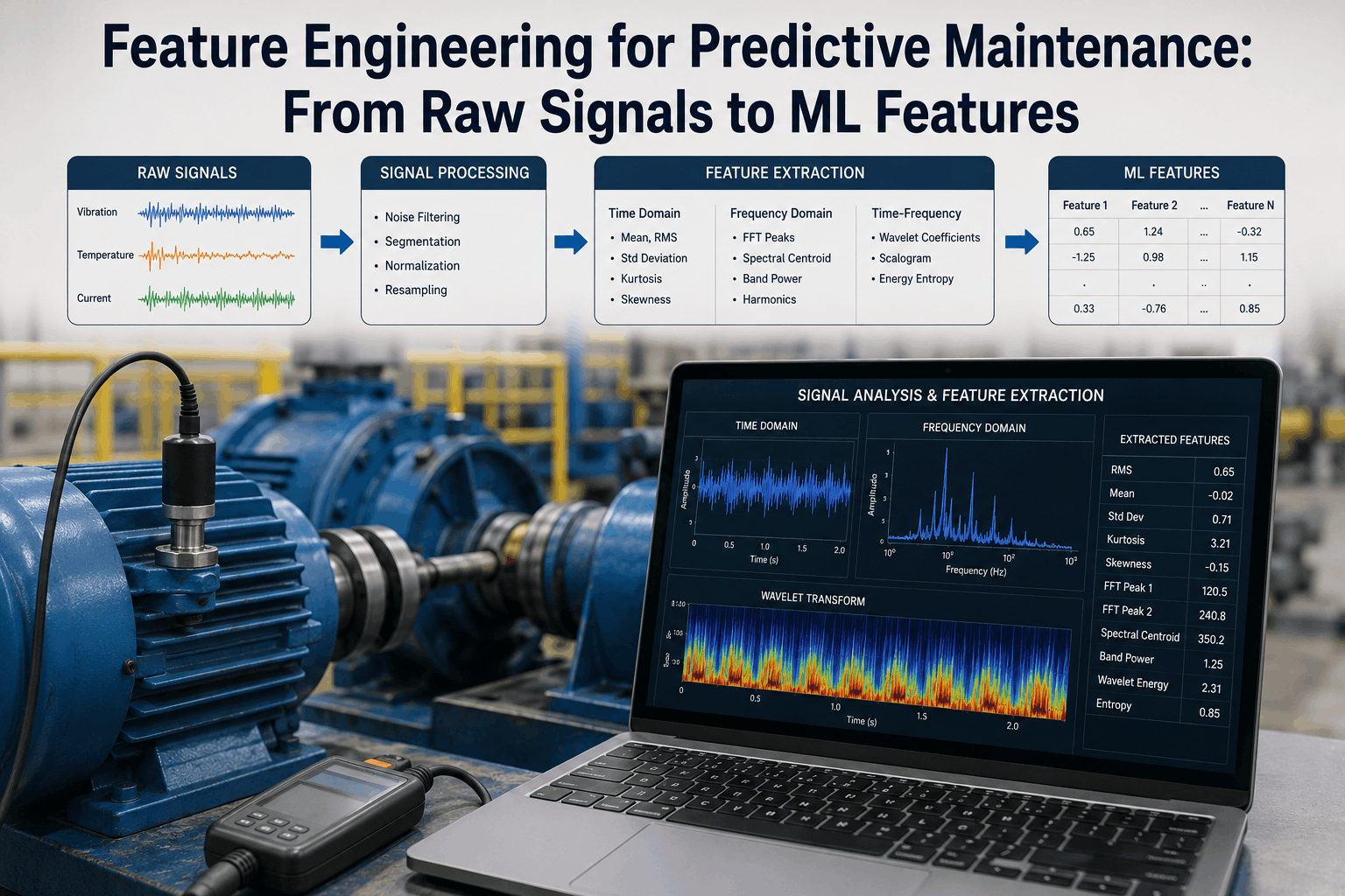
Raw sensor signals — vibration acceleration waveforms, motor current time series, temperature readings — contain the physical information that predicts equipment failure, but not in a form that machine learning models can directly exploit. Feature engineering is the process of transforming these raw signals into compact numerical representations that capture fault-relevant physics while discarding noise and irrelevant variation. The quality of feature engineering determines model accuracy ceiling regardless of how sophisticated the downstream ML algorithm is — a gradient boosting model trained on well-engineered features will consistently outperform a deep neural network trained on poorly extracted ones for industrial fault detection tasks. Get iFactory Support to deploy production-grade feature engineering pipelines on your industrial sensor data today.
Extract ML-Ready Features from Raw Vibration, Temperature, and Current Signals
iFactory's signal processing pipeline transforms raw industrial sensor data into fault-discriminative features — time-domain statistics, frequency-domain peaks, wavelet coefficients, and cross-signal ratios that ML models need to detect equipment degradation accurately.
The Three Signal Domains and Their Feature Families
Industrial sensor signals carry fault information across three complementary domains — time, frequency, and time-frequency — and the features most sensitive to specific fault types differ systematically across these domains. A complete feature engineering strategy covers all three domains, using domain knowledge to focus computation on the signal features most informative for the specific failure modes being modeled. Contact iFactory to configure a feature extraction pipeline calibrated to your specific sensor types and failure modes.
Domain 1
Time-Domain Statistical Features
Statistical moments and order statistics computed directly from the signal time series: RMS (proportional to signal energy), peak value, crest factor (peak/RMS — elevated by impulsive faults), kurtosis (4th moment — sensitive to transient impulsive events from bearing defects and gear damage), skewness, and shape factor. Time-domain features are computationally inexpensive, interpretable, and effective for fault severity quantification across vibration, current, and temperature signals.
Domain 2
Frequency-Domain Spectral Features
Features extracted from the Fourier transform of the signal: amplitude at theoretically predicted fault frequencies (bearing defect frequencies BPFO, BPFI, BSF, FTF; gear mesh frequency and sidebands; motor current harmonics), spectral centroid, spectral bandwidth, and spectral entropy. Frequency-domain features are fault-mechanism-specific — each fault type produces characteristic spectral components that distinguish it from other failure modes operating on the same machine.
Domain 3
Time-Frequency Features (Wavelet)
Wavelet transform and Short-Time Fourier Transform (STFT) provide joint time-frequency representations — capturing both when spectral changes occur and at what frequency. Wavelet packet decomposition coefficients at specific sub-band energy levels, scalogram-derived features, and STFT spectrogram statistical features are particularly valuable for non-stationary signals where fault signatures appear transiently rather than continuously in the frequency domain.
Domain 4
Envelope Analysis Features
Envelope analysis bandpass-filters the signal around a structural resonance frequency excited by impulsive fault events, then demodulates the envelope to extract the repetition rate of the impulses. Envelope spectrum features — amplitude at fault repetition frequencies like BPFO — are the most sensitive method for detecting early-stage bearing defects, where the fault impulse energy is spread across a wide frequency band but the impulse repetition rate produces a narrow envelope spectrum peak.
Domain 5
Cepstral Features
Cepstrum analysis converts the log power spectrum to the quefrency domain, where periodic families of sidebands appear as distinct peaks. Cepstral features are particularly effective for detecting gear tooth damage (which produces sideband families around GMF harmonics) and modulated signals from variable-load machinery where amplitude and phase modulation creates sideband structures that cepstrum isolates more cleanly than direct spectral analysis.
Domain 6
Cross-Signal and Derived Features
Features derived from combinations of multiple signals often carry more diagnostic information than individual signal features. The ratio of bearing outer race to inner race defect frequency amplitudes distinguishes defect location. Motor current-vibration cross-correlation identifies electrical versus mechanical fault causes. Temperature-power efficiency ratios detect thermal degradation independently of load variation. Cross-signal features require alignment of signals in time and consistent operating condition normalization before computation.
Fault-to-Feature Mapping: What to Extract for Each Failure Mode
Feature engineering decisions should be driven by fault physics — the mechanical or electrical mechanisms that generate each failure mode produce specific signal characteristics that informed feature selection targets. The table below maps the primary failure modes encountered in industrial equipment to the feature domains most sensitive to each. Book a demo to see iFactory's fault-to-feature mapping configured for your specific equipment types.
Scroll for more →
| Failure Mode | Primary Signal | Most Sensitive Features | Why This Feature Works |
|---|---|---|---|
| Rolling Bearing Defect | Vibration acceleration | Envelope spectrum at BPFO/BPFI, kurtosis, crest factor | Bearing defects produce impulsive repetitive signals at defect pass frequencies |
| Gear Tooth Damage | Vibration acceleration | GMF sideband amplitudes, cepstrum at shaft period, FM4 | Tooth damage modulates GMF amplitude and phase at shaft rotation frequency |
| Motor Winding Fault | Motor current (all 3 phases) | Negative sequence current ratio, 3rd/5th/7th harmonic amplitudes | Winding asymmetry creates negative sequence current and odd harmonic distortion |
| Broken Rotor Bar | Motor current | Sideband amplitudes at (1±2ks)f₁, slip-normalized | Broken bars create current sidebands at slip-dependent frequencies around fundamental |
| Pump Cavitation | Vibration + pressure | Sub-synchronous vibration, broadband noise floor, pressure fluctuation RMS | Cavitation generates broadband noise from bubble collapse plus sub-sync instability |
| Heat Exchanger Fouling | Temperature (multiple points) | LMTD efficiency ratio, approach temperature trend, thermal time constant | Fouling reduces heat transfer coefficient, increasing approach temperature at constant flow |
Feature Quality Metrics: Discriminability and Stability
Feature Discriminability (Fisher Score)
Target: Fisher Score ≥ 2.0
Fisher score measures how well a feature separates healthy from fault classes — the ratio of inter-class variance to intra-class variance. Features with Fisher score below 1.0 have overlapping healthy and fault distributions and contribute noise to the model. Features above 3.0 are highly discriminative and should be prioritized in model training. Computing Fisher scores across all candidate features guides which features to include in the final feature set.
Feature Stability Under Load Variation
Target: CoV < 15% at Constant Health
A feature that changes with operating load rather than fault state creates false positive detections when load increases and false negative misses when load decreases. Coefficient of variation (CoV = standard deviation / mean) measured across multiple load conditions on a confirmed-healthy asset quantifies feature stability. Features with CoV above 25% at constant health require load normalization before use as fault indicators.
Feature Monotonicity (Trend Consistency)
Target: Monotonicity Score ≥ 0.7
For remaining useful life prediction, features should trend consistently in one direction as degradation progresses — increasing (like kurtosis during bearing degradation) or decreasing (like efficiency during fouling). Monotonicity score measures the fraction of consecutive time step pairs where the feature moves in the consistent direction. Low monotonicity features are noisy trend indicators that produce unstable RUL estimates even when the overall trend is correct.
Feature Dimensionality After Selection
Target: 15–40 Features per Model
Unconstrained feature extraction from a single vibration sensor can generate hundreds of candidate features. Including all of them in a model introduces the curse of dimensionality — model variance increases, training time grows, and interpretability decreases. Feature selection (Fisher score ranking, mutual information, recursive feature elimination) identifies the 15–40 features that carry the most non-redundant fault information for each specific failure mode model.
Signal Processing Pipeline: From Raw Acquisition to Feature Vector
Signal Conditioning and Preprocessing Foundation Step
Raw sensor signals require conditioning before feature extraction: anti-aliasing filtering to prevent spectral aliasing, DC offset removal (high-pass filtering at 2–5 Hz), amplitude calibration against sensor sensitivity specifications, and synchronization of signals from different sensors to a common time base. Missing value imputation handles sensor dropouts — linear interpolation for short gaps (under 5% of window length), window exclusion for longer gaps. Signal quality scoring flags windows with excessive noise floor elevation or clipping that invalidate feature extraction.
Operating Condition Normalization
Many time-domain and frequency-domain features vary with operating conditions (speed, load, temperature) independently of fault state. Speed normalization using order tracking resamples the vibration signal from time domain to shaft-revolution domain — making all spectral features independent of speed variation. Load normalization divides feature values by a reference load metric (power draw, flow rate, pressure). Without normalization, load changes produce false positive alerts and load reductions produce false negative misses.
Time-Domain Feature Extraction
Statistical features computed from the conditioned time-domain signal within each analysis window: RMS, peak, peak-to-peak, crest factor, kurtosis, skewness, shape factor, impulse factor, and margin factor. Window length selection balances temporal resolution against statistical estimation accuracy — longer windows produce more stable estimates but lower temporal resolution for detecting rapid degradation onset. Typical window lengths: 1–5 seconds for rotating machinery (capturing 50–250 revolutions at 3,000 RPM).
Frequency-Domain Feature Extraction
FFT of each analysis window produces the power spectrum from which fault-frequency-targeted features are extracted: amplitude at bearing defect frequencies (BPFO, BPFI, BSF, FTF for vibration; (1±2ks)f₁ for current), GMF harmonics and sidebands for gearbox vibration, and spectral statistics (centroid, bandwidth, entropy, spectral kurtosis). Frequency resolution is determined by FFT length — longer FFTs provide finer frequency resolution but require longer signal segments.
Wavelet and Envelope Feature Extraction
Wavelet packet decomposition at 3–5 levels provides sub-band energy features that track fault energy distribution across frequency bands without requiring prior knowledge of exact fault frequencies. Envelope analysis uses the kurtogram or spectral kurtosis to identify the optimal bandpass filter center frequency and bandwidth for demodulation — automating the filter selection process that traditionally required manual expert selection. Wavelet and envelope features complement FFT features for detecting early-stage transient faults not yet visible in the average spectrum.
Feature Selection and Dimensionality Reduction
The full extracted feature set — potentially 200–500 features from all domains — is reduced to a compact, non-redundant subset using filter-based selection (Fisher score, mutual information), wrapper-based selection (recursive feature elimination with the target model), and correlation-based redundancy elimination (removing features with pairwise correlation above 0.85). The final feature set of 15–40 features feeds the downstream ML model with minimal redundancy and maximum fault discriminability. Contact iFactory Support to configure automated feature selection for your specific fault detection task.
Feature Engineering Infrastructure Requirements
Edge FFT Processing
On-device FFT computation at 10–20kHz sampling rates — iFactory edge hardware performs spectral analysis locally to reduce data transmission bandwidth by 100–1000× versus transmitting raw waveforms to cloud
Fault Frequency Library
Pre-computed bearing defect frequencies, gear mesh frequencies, and motor fault frequencies for 50,000+ equipment models — auto-populating the target frequency list from asset nameplate data entry
Order Tracking Module
Tachometer-based order tracking resampling that normalizes vibration spectra for speed variation — enabling fault frequency detection across the full operating speed range without speed-induced false positives
Feature Drift Monitoring
Continuous monitoring of healthy-state feature distributions — alerting when feature statistics drift from the established healthy baseline in ways that indicate sensor degradation or operating condition change rather than equipment fault
Feature Engineering Implementation: 6-Phase Roadmap
01
Fault Physics Documentation
Before extracting any features, document the physical mechanism for each target failure mode and the signal characteristics it is expected to produce. Which signal type is most sensitive (vibration, current, temperature)? At what frequencies do fault signatures appear? Are they impulsive or continuous? This documentation drives feature domain selection and prevents wasted computation on uninformative features.
02
Fault Frequency Calculation
From equipment nameplate data (bearing model numbers, number of gear teeth, motor pole pairs, rated speed), calculate the theoretical fault frequencies for each failure mode. Enter these into iFactory's fault frequency library — the system automatically tracks amplitudes at these frequencies and their harmonics without requiring manual spectral inspection at each measurement cycle.
03
Candidate Feature Extraction on Labeled Data
Extract all candidate features from both labeled failure windows and confirmed-healthy windows. Compute Fisher scores across the full candidate feature set to identify which features show the strongest separation between healthy and fault classes. Visualize feature distributions for the top-20 features to validate that the separation is real rather than an artifact of labeling bias or operating condition confounding.
04
Operating Condition Normalization Validation
Verify that top-ranked features are stable under healthy-state operating condition variation. Extract features from periods of known-healthy operation at different load points and speed settings. Features whose values change substantially with operating conditions (CoV above 25%) require normalization before use as fault indicators — otherwise load changes produce false alarms.
05
Feature Selection and Final Set Definition
Apply recursive feature elimination with cross-validation using the target model architecture to identify the final feature set. Start with the top-50 features by Fisher score, apply correlation-based redundancy elimination, then use wrapper-based selection to identify the subset that maximizes validation set AUC-PR. Document the final feature set definition for reproducibility and production pipeline configuration.
06
Production Pipeline Deployment and Monitoring
Deploy the production feature extraction pipeline and implement continuous monitoring of feature statistics. Feature distribution drift — the shift of healthy-state feature distributions over time from sensor aging, process changes, or equipment modification — must be detected and addressed to maintain model accuracy. iFactory monitors feature health metrics continuously and alerts when drift exceeds thresholds that would require model retraining. Get iFactory Support to deploy your production feature pipeline.
Frequently Asked Questions
Do deep learning models eliminate the need for feature engineering?
Deep learning models can learn feature representations automatically from raw signals — convolutional networks on raw waveforms or spectrograms have shown strong performance on benchmark datasets like C-MAPSS. However, in industrial deployments with scarce labeled data, hand-engineered physics-informed features consistently outperform end-to-end deep learning because they encode domain knowledge that would require orders of magnitude more training examples for a deep network to discover. A practical approach is to combine engineered features as inputs to a classical ML model for reliable production performance, while using deep learning for exploratory feature discovery that may identify new informative representations.
How should feature extraction window length be selected?
Window length involves a fundamental tradeoff between statistical estimation accuracy and temporal resolution. Longer windows produce more stable feature estimates (lower variance from random noise) but reduce the temporal resolution for detecting fault onset. A practical guideline: minimum window length should capture at least 50 shaft revolutions for rotating machinery (ensuring adequate frequency resolution for fault frequency detection), with typical industrial applications using 1–10 second windows at 3,000–1,500 RPM respectively. For variable-speed machinery, minimum revolution count rather than fixed time is the correct specification.
What is the difference between spectral kurtosis and the kurtosis used in time-domain feature extraction?
Time-domain kurtosis measures the impulsiveness of the overall signal time series — a single number summarizing the statistical character of the waveform. Spectral kurtosis (and its frequency-domain visualization, the kurtogram) measures the kurtosis of the signal's instantaneous amplitude at each frequency — producing a frequency-dependent kurtosis spectrum that identifies which frequency bands contain the most impulsive content. Spectral kurtosis is used to select the optimal bandpass filter center frequency and bandwidth for envelope analysis, rather than as a direct fault indicator itself.
How does iFactory handle feature extraction for variable-speed equipment?
Variable-speed equipment requires order tracking — resampling the vibration signal from the time domain to the angular domain (revolutions) so that all spectral features are computed in terms of shaft orders rather than Hz. This makes fault frequencies (which are proportional to shaft speed) appear at constant positions in the order spectrum regardless of operating speed. iFactory's order tracking module uses tachometer pulse input to perform the angular resampling automatically, enabling fault frequency tracking across the full operating speed range without speed-induced spectral smearing.
Build the Feature Engineering Pipeline That Determines Your Model's Accuracy Ceiling
iFactory's signal processing toolkit extracts fault-discriminative features from raw vibration, current, and temperature signals — combining time-domain statistics, frequency-domain fault tracking, wavelet decomposition, and cross-signal ratios into the feature vectors that make PdM models actually work in production.