Every AI vision model needs data. Thousands of labeled images per defect class — good parts, bad parts, borderline cases, lighting variations, material batches, and edge conditions. A factory that has been running for two years has this data. A greenfield factory on commissioning day has exactly zero images. This is the cold-start problem, and it kills more AI vision deployments than any technical challenge. Without a training data strategy, the factory has two choices: run without AI inspection for 3-6 months while collecting production images (shipping defects to customers the entire time), or deploy a model trained on generic data that produces 15-30% false positive rates (destroying operator trust in the system within the first week). Both options are unacceptable. In twenty years of deploying AI vision in manufacturing, I've developed a systematic approach that solves the cold-start problem: synthetic defect generation from product CAD creates realistic training images before the first part is produced, transfer learning from models trained on similar products provides a pre-trained feature extractor, and day-one deployment with conservative thresholds ensures the system catches real defects while minimizing false alarms. The result: 95%+ detection accuracy from the first production shift, improving to 99.5%+ within 90 days as real production data replaces synthetic data through an active learning pipeline. No waiting. No shipping defects. No operator trust destruction. Schedule a Demo
The Cold-Start Problem
Don't wait 9-12 months for your AI vision to work. Schedule a demo to see how synthetic data and transfer learning deliver 95%+ accuracy from your first production shift.
Synthetic Defect Data Generation
Product CAD to Rendered Images
Product 3D CAD model rendered under simulated camera and lighting conditions matching the actual inspection station design. Physically-based rendering (PBR) generates photorealistic images with accurate material reflectance, surface texture, and shadow patterns. Camera parameters (focal length, sensor size, working distance, lens distortion) matched to the specified inspection hardware. Output: 10,000+ images of good parts with realistic variation in positioning, orientation, and surface finish.
Defect Injection Engine
Known defect types from the product defect specification (scratches, dents, porosity, discoloration, cracks, contamination) procedurally injected onto rendered good-part images. Defect parameters randomized within physically plausible ranges: size (0.05-5mm), depth (surface to subsurface), orientation (0-360°), location (random across inspectable surfaces), and appearance (color, texture, reflectivity). Each defect type generated with 5,000-10,000 variations. Result: 50,000+ labeled synthetic defect images before the first real part exists.
Domain Randomization
Lighting intensity varied ±20%, camera angle perturbed ±3°, background texture randomized, surface finish variation added (matte to glossy range), and noise injected to simulate real camera sensor noise. This forces the AI model to learn defect features — not background patterns or lighting artifacts. Domain randomization is the key to synthetic-to-real transfer: models trained on heavily randomized synthetic data generalize 40-60% better to real production images than models trained on clean synthetic data alone.
Validation Against Real Samples
Before production, sample parts from pilot runs or prototype builds are inspected under the actual camera and lighting setup. These real images (even 50-100 images) are used to validate that the synthetic data distribution matches reality. If the domain gap is too large (accuracy drops >10% on real vs synthetic test set), the rendering parameters are adjusted. This validation step ensures the synthetic model will transfer effectively to production. Without validation, synthetic-only models risk a domain gap that undermines day-one accuracy.
Transfer Learning Architecture
Day-One Deployment: Conservative Threshold Strategy
High Sensitivity, Low Specificity
Day-one model deploys with detection thresholds set conservatively: the model flags anything remotely suspicious. This means a higher false positive rate (5-10% vs the eventual 0.5-2%) but near-zero false negatives — real defects are caught. Operators review flagged items and confirm/reject. This is deliberate: it's far better to over-inspect on day one than to miss defects. Operator trust is built by catching real defects consistently — even if they also review some false alarms.
Uncertainty-Based Flagging
The model outputs not just a classification but a confidence score. Parts classified with >95% confidence are auto-passed or auto-rejected. Parts between 70-95% confidence are flagged for human review. Parts below 70% confidence are auto-rejected (conservative). This uncertainty-based routing ensures the model "knows what it doesn't know" — borderline cases get human oversight while clear cases are handled automatically. As the model improves, the uncertainty zone shrinks and automation increases.
Parallel Mode: First 72 Hours
For the first 72 hours, the AI system runs in parallel with manual inspection — both systems inspect every part, but only manual inspection drives accept/reject decisions. AI predictions are logged and compared against manual results. This builds a labeled dataset from production (AI prediction vs human ground truth), validates AI accuracy in real conditions, and gives operators confidence in the system before it goes live. After 72-hour validation: AI goes primary, manual becomes spot-check.
Escalation Protocol
When AI encounters a defect type not in its training data (a "novel defect"), it flags the image with "unknown defect — human review required." Novel defect images are immediately routed to a quality engineer for classification and added to the active learning queue. The model never silently passes an unknown defect type. This escalation protocol ensures that even the most unusual manufacturing anomalies are caught — not by the AI, but by the human-AI collaboration system designed around the AI's known limitations.
Want a day-one AI deployment strategy for your greenfield facility? Schedule a demo to see how conservative thresholds and active learning deliver reliable inspection from the first shift without destroying operator trust.
Active Learning: 30/60/90 Day Plan
Every image flagged for human review becomes a labeled training sample. Operators confirm or correct AI predictions on the HMI touchscreen — 5-10 seconds per image. Target: 5,000-10,000 real labeled images in 30 days. Model retrained nightly with real production data mixed into the synthetic+transfer training set. Accuracy improvement: 95% → 97%+. False positive rate drops 50% as model learns normal production variation (lighting shifts, surface finish batch variation, positioning tolerance).
Active learning algorithm identifies the most informative unlabeled images — images near decision boundaries where the model is least confident. These are prioritized for human labeling over easy cases. This targeted approach builds accuracy where it matters most: borderline defects that are hard to classify. Model begins seeing rare defect types as production volume accumulates. Accuracy: 97% → 98.5%+. Synthetic data proportion in training set drops below 30% as real data dominates.
Model has seen 20,000-50,000 real production images covering the full range of normal variation and defect types. Synthetic data used only for rare defect augmentation. Final accuracy: 99.5%+. False positive rate: <0.5%. False negative rate: <0.1% for known defect types. Model validated against held-out test set with formal accuracy report. Model version frozen and deployed as "production baseline." All subsequent updates go through model governance process.
Data Labeling Workflow & Quality Assurance
Every inspection image saved with metadata: timestamp, product serial, camera ID, lighting recipe, AI prediction, confidence score. Images automatically sorted into queues: auto-labeled (high confidence), review-needed (medium confidence), novel (unknown class). Storage: 50-200 GB/day depending on resolution and product volume.
Level 1: Operator confirms/rejects AI prediction on HMI (5-10 sec/image). Level 2: Quality engineer reviews and relabels flagged disagreements (30-60 sec/image). Level 3: Senior quality or external expert validates edge cases and novel defects (2-5 min/image). Inter-annotator agreement tracked: >95% agreement required for label to be accepted into training set.
Random 5% sample of all labels reviewed by Level 2 annotator for consistency. Systematic errors detected: if operator X consistently mislabels defect type Y, retraining is triggered for that operator. Label conflict resolution: disagreements between annotators escalated to quality engineer. All labels version-controlled — every change tracked with annotator ID and timestamp.
New labeled images merged into training dataset. Model retrained overnight on GPU cluster. New model validated against held-out test set. If accuracy improves: new model staged for review. If accuracy degrades: new data inspected for labeling errors. Human approval required before any model version is promoted to production. Full audit trail: training data → model version → validation results → approval signature.
Model Governance & Versioning
Version Control
Every model version tracked with: training data hash, hyperparameters, validation accuracy, approval signature, deployment timestamp, and rollback capability. Model registry stores all versions — any previous version can be redeployed in under 5 minutes if a new version shows unexpected behavior in production. Git-like branching for experimental models vs production models.
Validation Protocol
Before any model version goes to production: tested against a held-out golden test set (500-1,000 images, never used in training, refreshed quarterly). Accuracy, precision, recall, and F1-score per defect class reported. Regression test: new model must match or exceed previous version on every metric. A/B testing: new model runs in shadow mode (predictions logged but not acted on) for 24-72 hours before promotion.
Drift Detection
Production model accuracy monitored continuously. Statistical process control (SPC) on model confidence scores — a sustained shift in confidence distribution signals data drift (new material, lighting change, process adjustment). Automated alert triggers investigation and potential retraining. Quarterly model review: formal assessment of accuracy vs deployment targets with documented action items.
Audit Compliance
Full traceability for regulated industries: which model version inspected which product, what training data was used, who approved the model, what accuracy was achieved. Meets requirements for IATF 16949 (automotive), AS9100 (aerospace), ISO 13485 (medical), and 21 CFR Part 11 (FDA). Audit-ready documentation auto-generated per model version — no manual report preparation before audits.
Key Benefits & ROI
Day One AI Accuracy Is Not Magic. It's Planning.
iFactory designs the complete AI training data strategy for greenfield deployments — synthetic data generation, transfer learning, day-one conservative deployment, active learning pipelines, and audit-compliant model governance — so your AI vision system catches defects from the first production shift.
Frequently Asked Questions
Don't Ship Defects While Your AI Learns
Every day without AI inspection is a day defects escape to customers. Synthetic data + transfer learning + conservative deployment = 95%+ accuracy from shift one. Zero excuses for waiting.