Static control limits in aerospace composite layup have a measurable shelf life that most operations do not track and few manage proactively. The UCL and LCL calculated during the AS9100 qualification study reflect the process state that existed across those 25 to 30 subgroups — specific compaction roller condition, specific prepreg batch, specific ambient temperature range, specific operator technique. AFP compaction rollers wear 0.1 to 0.3 mm over 500 hours of production. Prepreg tack varies significantly between lot numbers. Factory floor temperature in a non-conditioned layup cell can shift 8 to 12 degrees Celsius between summer and winter production schedules. The static limits do not change. They remain anchored at the qualification values while the process distribution shifts, widens, narrows, and drifts around them. The gap between what the control chart shows and what the process is actually doing grows wider with every variable that enters production — producing both missed signals and false alarms as the limits become progressively misaligned with the current process state. Adaptive control limits close this gap by treating UCL and LCL as live parameters that self-tune continuously, keeping detection sensitivity aligned with the process as it exists today rather than as it existed at qualification.
Adaptive Control Limits · AI-Native SPC · Cpk Sustainability
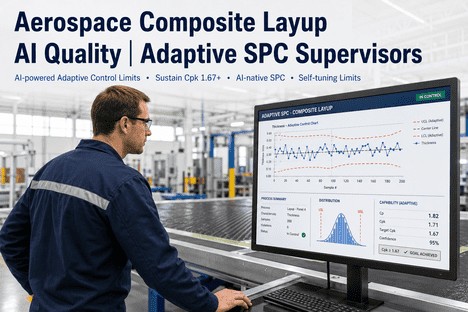
Static Limits Stay Where You Put Them. The Process Moves. Adaptive Limits Move With It.
ML-driven adaptive UCL/LCL replace static qualification-era limits with live boundaries that self-tune as AFP tooling wears, material batches change, and environmental conditions shift — sustaining Cpk 1.67+ through every phase of production.
Why Static Limits Lose Relevance: The 12-Month Decay Cycle in AFP Composite Layup
A control limit calculated from qualification data is a snapshot of the process at one point in time. Composite layup is not a static process — it is a dynamic system where tooling condition, material properties, environmental factors, and operator technique all evolve across a production programme. The timeline below shows how static limits progressively lose relevance over a typical 12-month production cycle, and why adaptive limits maintain detection accuracy throughout.
UCL and LCL calculated from 30 subgroups of stable process data. Process deemed capable at Cpk 1.67. Limits accurately reflect the current process state. Adaptive and static limits are identical at this point.
Compaction roller wear reaches 0.08 mm. Prepreg lot transitions to batch B with slightly different tack characteristics. Process mean shifts 0.15 sigma. Static limits do not shift. Adaptive limits begin tracking the new centreline. Detection gap opens.
Accelerated Drift — Month 6
Seasonal temperature shift of 6 degrees Celsius changes material behaviour. Static limits now lag the actual process distribution by 0.4 sigma. First false alarm from static system as process narrows. Adaptive limits maintain alignment with current variance.
Critical Misalignment — Month 9
Gap between static UCL and actual 99.7% percentile exceeds 0.8 sigma. Process drift in gap width goes undetected by static limits. Adaptive limits flag the developing trend at 0.25 sigma via Western Electric rule 5. Static limits show nothing.
Scrap Event — Month 10-12
Post-cure inspection rejects 3 panels from the same production run. Root cause investigation traces the failure to gap-width drift that began at month 5 and crossed the specification limit at month 10. Static limits never fired. Adaptive limits detected the trend at month 5 — five months before the first scrap panel.
Qualification is not a permanent badge of capability. It is a certificate of process state on the day of testing. The process changes. If the limits do not change with it, the control chart becomes a compliance artefact rather than a prevention tool. Adaptive control limits are not a replacement for qualification — they are a mechanism for keeping qualification-era limits relevant across the full production lifecycle.
— Lead Quality Engineer, Aerospace Tier 1 Composite Structures
What Adaptive Control Limits Actually Do
Adaptive control limits use machine learning algorithms to continuously recalculate UCL, LCL, and centreline as new measurement data arrives. The ML model evaluates the current process distribution against its recent history — typically a rolling window of 50 to 200 subgroups — and updates the limits to maintain the appropriate detection sensitivity for the current process state. This is not a simple moving average. The model distinguishes between common-cause variation that should widen the limits and special-cause variation that should trigger an alarm. It detects shifts in process mean and variance independently, and it adjusts limits at different rates for different parameters based on each characteristic's natural behaviour pattern. The result is a control chart where the limits reflect what the process is doing now, not what it was doing at qualification.
For the AFP composite layup supervisor, this means every signal on the chart is a genuine signal. False alarms from stale limits disappear. Drift detection begins at the point of onset rather than at the point of limit breach. Cpk values on the dashboard are calculated against current adaptive limits, not qualification-era static limits — giving a true picture of process capability at the moment of measurement. The supervisor stops spending time investigating alarms that turn out to be limit misalignment and starts spending time on the patterns that actually indicate process degradation.
Static SPC vs Adaptive SPC: What Changes for the Supervisor
The operational difference between static and adaptive SPC is not theoretical. It directly affects how supervisors spend their time, what signals they act on, and whether the control chart prevents scrap or merely documents it. The comparison below shows the practical difference across six dimensions that matter on the AFP cell floor.
✗
Limits fixed at qualification — unchanged for 6-12 months regardless of process evolution
✗
Detects only single-point ±3-sigma breaches — misses runs, trends, and patterns entirely
✗
False alarms when process variance narrows; missed signals when process mean shifts
✗
Cpk reported monthly — by the time the report arrives, the capability data is already stale
✗
Supervisor investigates 60%+ false alarm rate — most alarms are limit misalignment, not process issues
✗
Requires manual limit recalculation — every limit update consumes 4-8 hours of engineering time
✓
Limits self-tune with every subgroup — UCL/LCL reflect current process distribution continuously
✓
All eight Western Electric rules evaluated automatically — trend detection at 0.25 sigma resolution
✓
Appropriate sensitivity at all times — limits widen or narrow as process variance dictates
✓
Live rolling Cpk — capability visibility at the moment of measurement, not at month end
✓
Sub-10% false alarm rate — ML prioritisation ensures genuine signals reach the supervisor
✓
Zero-touch limit maintenance — limits update automatically without engineering intervention
The Cpk Sustainability Staircase: Climbing from 1.0 to 1.67+
Process capability index (Cpk) is not a static property of a manufacturing process. It is a time-dependent metric that degrades as the process drifts away from the qualification baseline. Static SPC allows this degradation to happen silently between monthly capability studies. Adaptive SPC maintains Cpk by keeping control limits aligned with current process conditions, enabling early intervention before capability erodes. The staircase below shows the capability progression that adaptive limits enable.
Cpk 1.67+
Sustained near-zero defect rate with adaptive limits tracking every process shift. Defect rate below 1 ppm. Limits self-tune to maintain constant detection sensitivity regardless of process variation.
Cpk 1.50
Process optimised with adaptive limits maintaining alignment. Occasional minor drift detected early and corrected. Defect rate below 7 ppm. Limits update weekly to track gradual tool wear.
Cpk 1.33
Process capable with static limits still adequate. Detection sensitivity beginning to degrade as limits lag process evolution. Defect rate around 64 ppm. Manual limit review needed quarterly.
Cpk 1.17
Process showing early capability erosion. Static limits missing approximately 30% of developing drift signals. Defect rate rising toward 300 ppm. Adaptive limits begin showing value at this threshold.
Cpk 1.00
Baseline static SPC at qualification. Limits accurate at this point but will degrade as process evolves. Defect rate around 1,350 ppm. First-pass yield approximately 93%. No adaptive mechanism in place.
Four Mechanisms That Make Adaptive Limits Work in Composite Layup
Adaptive control limits are not a single algorithm. They are a system of four coordinated mechanisms that work together to maintain detection accuracy as the process evolves. Each mechanism addresses a specific failure mode of static SPC in composite layup.
M1
Rolling Window Recalculation
UCL and LCL are recalculated from a rolling window of the 100 most recent subgroups. As new data enters the window, the oldest data exits. The limits automatically track gradual process evolution — tool wear, material drift, seasonal shifts — without requiring manual intervention. The window width is configurable per parameter: stable characteristics use wider windows for smoother limits; dynamic characteristics use narrower windows for faster adaptation.
M2
EWMA Centreline Tracking
Exponentially weighted moving average continuously tracks the process centreline, giving greater weight to recent measurements while retaining a memory of historical behaviour. The EWMA lambda parameter controls adaptation speed — lower values produce smoother centrelines that reject noise; higher values enable rapid response to genuine process shifts. The system auto-tunes lambda per parameter based on observed process dynamics.
M3
Variance Stabilisation Logic
Static SPC treats variance as constant between limit updates. Adaptive SPC tracks variance as an independent time-series, detecting changes in process spread separately from changes in process mean. When variance increases — as it does during AFP head wear progression — the adaptive limits widen appropriately to maintain false alarm rates. When variance decreases — as it does after preventive maintenance — the limits narrow to improve detection sensitivity.
M4
Multi-Parameter Cross-Correlation
The ML model monitors correlations between multiple process parameters — gap width, tow angle, compaction force, and layup speed — and adjusts individual control limits based on cross-parameter behaviour. A shift in gap width that correlates with a known compaction force adjustment is treated differently from an uncorrelated gap width shift. This prevents unnecessary alarms during intentional process adjustments while maintaining sensitivity to genuine anomalies.
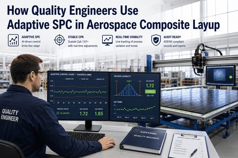
How Supervisors Use Adaptive Limits on the AFP Cell Floor
Adaptive control limits change the supervisor's relationship with the control chart. Instead of checking once per shift whether any points exceed the static UCL, the supervisor interacts with a live dashboard that surfaces the most important signals first. The daily workflow collapses to three focused actions.
STEP 1
Review Priority Queue
The dashboard presents the top 3 to 5 alerts ranked by business impact. Each alert includes the parameter, current value, trend direction, and recommended corrective action. Supervisors review the queue at shift start and at each production milestone. Average review time: 4 minutes.
STEP 2
Investigate Trend Context
One click opens the full control chart for the flagged parameter with adaptive limits, static limits overlaid, and the Western Electric rule that triggered the alert. The supervisor sees exactly when the trend began, which passes are affected, and whether correlated parameters show the same pattern.
STEP 3
Log Disposition or Escalate
For confirmed drift, the supervisor logs a corrective action request directly from the alert. The system tracks time-to-response and time-to-correction for each alert. Monthly reports show the supervisor's drift-detection-to-correction cycle time, false alarm rate, and contribution to Cpk sustainability.
Four Mechanisms · Rolling Window · EWMA · Variance Tracking
The Control Limits on Your Chart Are Still Set to Last Year's Process. The Process Changed. The Limits Did Not.
iFactory adaptive SPC replaces static qualification-era limits with self-tuning UCL/LCL that evolve with your AFP process — sustaining Cpk 1.67+ through tool wear, material transitions, and environmental variation. See it running on your process data.
Deploying Adaptive SPC on Your AFP Cell
Transitioning from static to adaptive SPC does not require replacing existing quality systems or re-qualifying the process. The adaptive layer runs alongside static control charts, providing supervisors with both views until the team gains confidence in the adaptive limits. The deployment pathway typically spans 8 to 12 weeks from data connection to full adaptive limit management.
1
Connect & Ingest
Connect to existing measurement data streams via OPC UA, MTConnect, or REST. No data migration required. Estimated duration: 1-2 weeks.
2
Phase I Baseline
Calculate provisional adaptive limits from 50-100 subgroups of historical data. Validate against known process events. Duration: 2-3 weeks.
3
Parallel Monitor
Run adaptive limits alongside static limits for 4-6 weeks. Compare alert quality and detection timing. Calibrate parameters per characteristic. Duration: 4-6 weeks.
4
Adaptive Go-Live
Transition to adaptive limits as primary control chart. Static limits retained for audit reference. Begin Cpk sustainability tracking with live rolling Cpk dashboard. Duration: 1 week.
Conclusion
Static control limits are not a quality system failure. They are a design limitation of a methodology developed in 1931 for a manufacturing environment where processes changed slowly and data arrived weekly. Aerospace composite layup in 2026 operates at a different pace — AFP heads layup at speeds where a single pass generates more data points than a week of production in Shewhart's era. The control limits that worked for static processes cannot keep pace with dynamic composite manufacturing where tooling wears, materials vary, and environmental conditions shift in real time.
Adaptive control limits address this gap by treating UCL and LCL as live process parameters that self-tune as the process evolves. The rolling window mechanism tracks gradual changes. The EWMA centreline responds to shifts at the right speed. The variance stabilisation logic maintains appropriate sensitivity as process spread changes. The cross-correlation model distinguishes intentional adjustments from genuine anomalies. Together, these four mechanisms keep control limits aligned with the actual process state — sustaining Cpk 1.67+ through every phase of production and eliminating the stale-limit detection gap that produces false alarms and missed signals in equal measure.
iFactory's adaptive SPC platform brings these four mechanisms together in a single interface designed for AFP composite layup supervisors — connecting to existing measurement systems, establishing initial adaptive limits from historical data, running alongside static charts during the validation period, and transitioning to full adaptive control with live rolling Cpk and pre-breach drift alerts. Book a Demo to see adaptive SPC configured for your AFP cell's process profile, or Talk to an Expert to discuss Cpk sustainability targets for your specific programme.
Frequently Asked Questions
The Control Limits on Your Dashboard Were Set for a Process That No Longer Exists. Adaptive Limits Track the Process You Have Right Now.
iFactory adaptive SPC for aerospace composite layup — self-tuning UCL/LCL, EWMA centreline tracking, variance stabilisation logic, and multi-parameter cross-correlation that sustains Cpk 1.67+ through every phase of production.