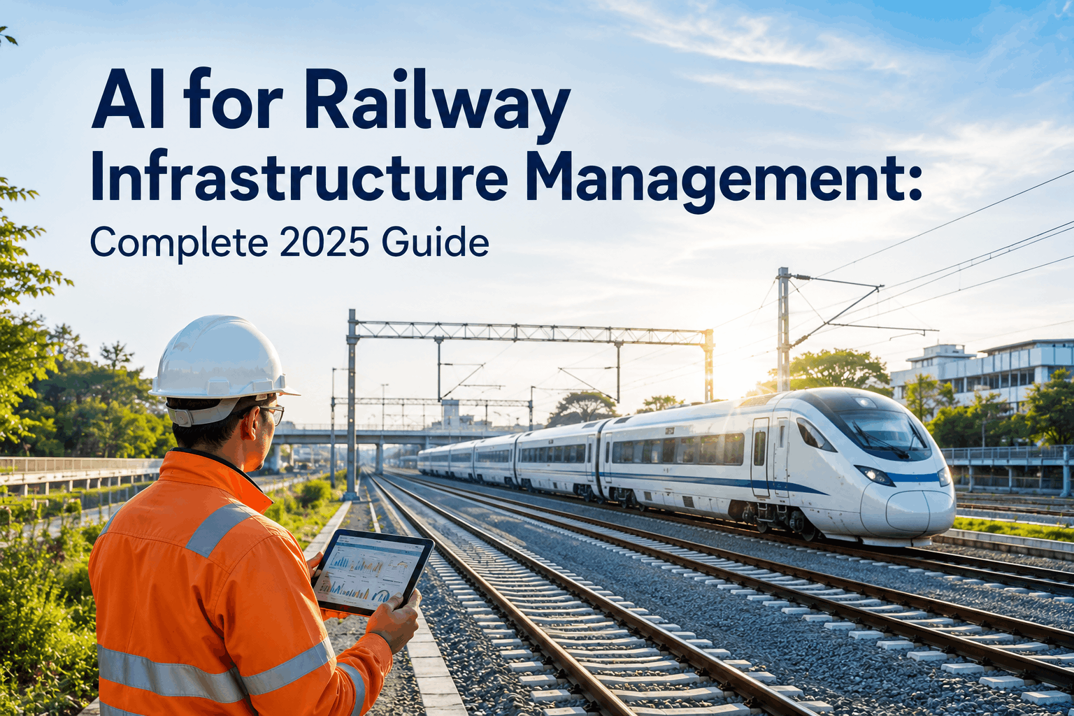
Every wheel that rolls over a rail joint, a worn fastener, a corrugated stretch, or a developing squat sends a unique vibration signature back up through the axle-box and into the bogie. Modern AI listens to that conversation continuously. By instrumenting in-service trains with axle-box accelerometers, carbody sensors, and microphones — and processing the signals through FFT, wavelet transforms, and deep convolutional networks — railway operators are now detecting track defects, fastener loosening, and subgrade settlement weeks before they become visible to manual inspection. Published research reports fastener defect classification accuracy of 98.27%, sub-millimetre detection of rail corrugation via microphone FFT, and reliable identification of squats and joints from axle-box acceleration on real Swedish and German rail networks. This article walks through how vibration analysis AI actually works on a working railway — the sensors, the signal processing, the ML architectures, and the defect categories each can detect. Book a Demo to see iFactory's vibration analytics pipeline running on live rail track today.
Technical Article · Vibration AI for Rail Track
Listening to Rail Track — One Axle-Box Vibration at a Time.
iFactory transforms axle-box vibration data into actionable maintenance intelligence — detecting corrugation, squats, fastener loosening, and subgrade settlement on in-service trains across the UK, EU, and MENA rail networks.
98.27%
Fastener defect classification accuracy reached by CNN on axle-box vibration data
3-axis
Vertical, lateral, and longitudinal acceleration — required for full track diagnostics
In-service
Sensors mounted on revenue trains — no dedicated inspection runs needed
Real-time
Edge processing detects defects as the train rolls over them
The Vibration Signal Processing Chain
From raw acceleration to actionable maintenance alert — a four-stage signal-processing pipeline. Each stage transforms the data into a more useful form for AI to interpret.
01
Raw Acquisition
Axle-box accelerometers sample at 1–10 kHz across vertical, lateral, and longitudinal axes. GPS and tachometer data sync each sample to a precise track location.
→
02
Preprocessing
Bandpass filtering, anti-aliasing, and noise reduction. Vold-Kalman filters decompose the signal into wheel-related and track-related components.
→
03
Feature Extraction
FFT and wavelet transforms generate frequency-domain features. RMS, kurtosis, and crest factor compute time-domain statistics. Spectrograms feed image-based models.
→
04
AI Classification
CNN, FCN, and recurrent architectures classify the signature into defect categories with confidence scores — feeding maintenance work orders directly to CMMS.
Frequency-Band Defect Mapping — What Each Frequency Range Reveals
Different track defects produce vibration signatures in different frequency bands. AI models learn to identify which band carries which fault — and how loudly.
Frequency Band
Primary Defect Detected
Typical Signal Source
Detection Method
0–20 Hz
Track geometry irregularity, subgrade settlement
Carbody acceleration, low-pass axle-box
Cross-correlation analysis, statistical features
20–100 Hz
Rail joints, switches, turnouts
Axle-box vertical and lateral acceleration
CNN on spectrograms, event-based classification
100–500 Hz
Squats, surface defects, isolated rail damage
Axle-box acceleration with high sample rate
1D CNN, time-frequency feature classifier
500 Hz – 2 kHz
Rail corrugation, head checking
Microphone, high-frequency accelerometer
FFT analysis on microphone signal
2–5 kHz
Fastener defects, bolt loosening, clip wear
Axle-box acceleration spectrum
Deep CNN on frequency-spectrum images
The Six Track Defects AI Reliably Detects from Vibration
Each defect category has its own ML maturity curve and characteristic detection accuracy in real-world deployment.
01
Rail Corrugation
Wave-like wear on the rail head. Detected via FFT on microphone signal — peak frequencies map directly to corrugation wavelength.
Maturity: Production
02
Squats & Surface Defects
Localised rail head damage. Axle-box acceleration produces a characteristic transient signature classifiable by CNN.
Maturity: Production
03
Fastener Defects
Loose, worn, or missing clips and bolts. CNN on frequency-spectrum images of axle-box vibration achieves 98.27% classification accuracy.
Maturity: Production
04
Joints & Turnouts
Worn or misaligned rail joints and switch components. Distinct event signatures detected via spatial-temporal correlation with GPS.
Maturity: Production
05
Subgrade Settlement
Ballastless track settlement detected via low-frequency carbody vibration patterns and ML classification.
Maturity: Emerging
06
Suspension Degradation
Worn dampers and stiffness loss inferred from multi-level vibration response — at wheelset, bogie, and carbody levels.
Maturity: Emerging
The ML Architectures Doing the Heavy Lifting
Four model families dominate vibration-based track health AI. Each plays a different role in the pipeline.
M1
1D Convolutional Neural Networks (1D CNN)
Operate directly on raw time-series acceleration data. Learn damage-sensitive features automatically without manual feature engineering. The standard for fastener clip health and squat detection.
M2
2D CNN on Spectrograms
Convert vibration signals to time-frequency images (spectrograms) and treat fault detection as an image classification problem. Achieves the 98.27% fastener accuracy benchmark from published Wiley research.
M3
Fully Convolutional Networks (FCN)
Take axle-box acceleration, track irregularity, and vehicle speed as simultaneous inputs — and predict fastener damage degrees with noise robustness validated on real network data.
M4
Vold-Kalman Filtering + ML Classifier
Signal decomposition into wheel-related and track-related components before classification. Enables track stiffness assessment and sleeper-passage analysis for predictive maintenance.
Where the Sensors Actually Go on a Train
Sensor placement determines what defects you can see. Production vibration AI uses a tiered sensor architecture across the train.
Position A
Axle-Box
Closest to the wheel-rail interface. The richest signal source for rail surface defects, fastener faults, and corrugation. Highest sample-rate sensors live here.
Position B
Bogie Frame
Mid-level vibration measurement — captures suspension behaviour and longer-wavelength track defects that propagate up from the wheelset.
Position C
Carbody
Lowest-frequency response. Captures large-scale track geometry irregularities, ride comfort metrics, and subgrade settlement signatures.
Position D
Interior Sensor-Box
Compact sensor box (accelerometers, gyros, microphones, GPS) deployed inside the carbody on multiple vehicle types — enabling network-wide monitoring at low cost.
From AI Output to Maintenance Trigger — The Threshold Logic
A vibration anomaly is not yet a maintenance work order. Production deployments apply a three-tier threshold model that converts AI outputs into action.
Tier 1 — Monitor
Below alert threshold
Anomaly logged for trend analysis. No action taken; pattern accumulates in the asset health timeline.
Tier 2 — Schedule
Alert threshold crossed
Maintenance work order auto-generated and scheduled into the next available possession window. Inspection priority elevated.
Tier 3 — Immediate
Critical threshold crossed
Real-time alert to control room. Speed restriction triggered if defect severity warrants. Engineering review within 30 minutes.
iFactory Vibration AI Platform
Make Every In-Service Train a Mobile Track Inspector.
iFactory's vibration analytics platform orchestrates axle-box, bogie, and carbody sensor data through Vold-Kalman filtering, FFT, wavelet, and CNN architectures — already deployed on live rail networks across the UK, EU, and MENA.
Trusted by track engineers, infrastructure managers, and rolling stock operators managing national rail networks.
Frequently Asked Questions
Tap any question to reveal the answer.
Vibration analysis AI detects six main categories of track defects from accelerometer and microphone data: rail corrugation (wave-like wear), squats and surface defects (localised rail head damage), fastener defects (loose, worn, or missing clips and bolts), joint and turnout wear, subgrade settlement, and suspension degradation. Each defect type produces a characteristic vibration signature in a specific frequency band — and modern CNN architectures learn to recognise these signatures with classification accuracy above 98% for fastener faults on published benchmarks. Book a demo to see live detection.
Three primary positions: axle-box accelerometers (closest to the wheel-rail interface, richest signal source), bogie-frame sensors (mid-level vibration capture for suspension and longer-wavelength defects), and carbody-mounted sensors (lowest-frequency response, captures ride comfort and track geometry). Some deployments add a compact sensor-box inside the carbody with combined accelerometers, gyroscopes, microphones, and GPS — enabling network-wide monitoring at low cost across multiple vehicle types. Axle-box accelerometers are the most diagnostic but require the highest sample rates.
Four architectures dominate. 1D CNNs operate directly on raw time-series acceleration and learn damage-sensitive features automatically. 2D CNNs convert vibration to spectrograms and treat fault detection as image classification — this is the architecture behind the 98.27% fastener accuracy benchmark. Fully Convolutional Networks (FCN) ingest axle-box acceleration, track irregularity, and vehicle speed simultaneously to predict fastener damage degrees. Vold-Kalman filtering combined with classifiers decomposes wheel-related and track-related signal components for track-stiffness assessment.
This is the core technical challenge in vibration-based track monitoring. The Vold-Kalman filter is the standard solution — it decomposes the raw signal into periodic wheel-related and track-related excitation-response pairs. Wheel out-of-roundness produces characteristic harmonics tied to rotation rate; track-related signals do not. Multi-level vibration measurement (at axle-box, bogie, and carbody) further helps separate the two — track signals propagate upward consistently, while wheel/suspension issues appear differently at each level.
Sample rate requirements depend on the defect being detected. Low-frequency defects (track geometry, subgrade settlement) work fine at 200–500 Hz sample rates. Mid-range defects (joints, squats) need 1–2 kHz. High-frequency defects (rail corrugation, fastener bolt vibration in the 500 Hz–5 kHz band) require 10 kHz or higher to satisfy Nyquist sampling. iFactory's standard deployment uses 10 kHz axle-box sensors and 1 kHz carbody sensors, covering the full defect spectrum with adequate resolution.
No — and regulators do not currently allow it to. Dedicated track recording cars and visual inspections remain mandatory under most rail safety regimes (UK ORR, EU ERA, FRA, etc.). What vibration AI does is augment those inspections: by running on in-service revenue trains, it provides continuous monitoring between mandated inspections, identifies emerging defects between scheduled measurement runs, and prioritises which sections need urgent attention. The combined approach delivers measurably better outcomes than either alone.
Real-world accuracy is typically 5–15% lower than published research benchmarks due to environmental noise, sensor drift, and the diversity of operational conditions not present in lab studies. Published fastener defect classification reaches 98.27% in controlled experiments. Production deployments on networks like Deutsche Bahn and Sweden's national rail typically deliver 88–93% accuracy after facility-specific model tuning. Continuous retraining on local data closes most of the gap within the first 6 months of operation.
iFactory connects natively to railway-industry CMMS and EAM platforms including SAP PM, IBM Maximo, Infor EAM, and national systems like Network Rail's Ellipse via standard REST APIs. Detected defects flow with their geo-referenced chainage, severity classification, and AI confidence score directly into the maintenance workflow. Work orders auto-generate against next available possession windows, and the digital twin updates with each inspection pass. There is no need to replace your existing planning stack.
Pilot deployment on a single train and one route typically completes in 6–10 weeks: sensor installation in 1–2 weeks, baseline data collection in 2–4 weeks, model calibration on facility-specific patterns in 2–4 weeks. Full multi-route, multi-train rollout extends to 16–24 weeks depending on fleet size. Most operators start with axle-box accelerometers on 5–10 trains covering primary corridors, then expand to fleet-wide deployment as the value case is proven and depot integration matures.