A bearing rarely fails silently. By the time the temperature rises, the vibration alarm trips, or the lube oil shows iron wear particles, the failure is already weeks deep. The earliest signal — the very first sign that something inside the machine is wrong — is usually acoustic. A 2 kHz harmonic creeps into the mel-spectrogram of a feed-pump motor that wasn't there last month. A faint 47 Hz modulation appears on a fan that's been running for ten years. A human ear walking the floor would notice some of these on a good day. A continuous CNN-LSTM autoencoder on every asset notices all of them, every shift, on a model trained on what your specific machine sounds like when it's healthy. iFactory's Acoustic + Vibration Anomaly stack puts an industrial microphone (or taps the existing accelerometer) on each critical asset, streams audio at 16 kHz to an NVIDIA Jetson AGX Orin edge gateway, computes mel-spectrograms in a 2-second sliding window, and runs a CNN-LSTM autoencoder that flags every spectral region the model can't reconstruct from learned-normal. Reconstruction-error map on the dashboard. CMMS work order auto-drafted on threshold breach. The model trains on the on-prem NVIDIA RTX PRO 6000 Blackwell + GB300 stack; inference runs at the edge in milliseconds. Live in 6 weeks from PO. See the full pipeline running on a real bearing rig at the iFactory booth, SAP Sapphire Orlando, May 11–13, 2026 — register here.
Acoustic + Vibration CNN-Autoencoder
Hear A Bearing Fail Weeks Before It Trips
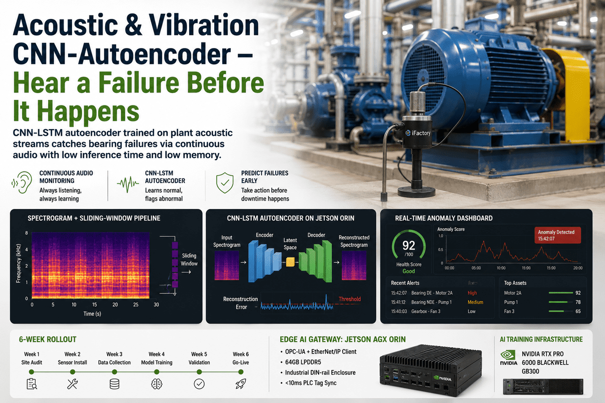
Industrial microphones and IEPE accelerometers stream audio and vibration at 16–25.6 kHz to NVIDIA Jetson AGX Orin gateways. Mel-spectrograms computed in 2-second sliding windows. CNN-LSTM autoencoder reconstructs each window from a model of your machine's healthy sound. Reconstruction error above the learned threshold flags an anomaly within 100 ms. Heatmap on the dashboard. Work order drafted in your CMMS. Engineer reviews. Operator commits. The AI never writes to the PLC.
The Failure Was Audible Before It Was Measurable — Vibration Trips Are Late Signals
Conventional condition monitoring waits for the RMS vibration value to cross a threshold. By that point the bearing race is spalled, the fan blade is cracked, or the gear tooth is chipped. Acoustic monitoring catches the same fault weeks earlier because the spectral fingerprint changes long before the energy magnitude does. A new harmonic at a bearing's ball-pass frequency, a faint cavitation hiss in a pump volute, a subtle modulation from a loose stator winding — all of these show up on the mel-spectrogram while the overall vibration RMS is still inside its alarm band. Talk to our acoustic AI lead about which assets on your floor would benefit most.
Vibration trip at 7.1 mm/s. Bearing already at end-of-life. Trip is the warning, not the early-warning. The acoustic content has been screaming for weeks but nobody was listening because the only metric tracked was the integrated magnitude. Most failures arrive as surprises this way.
The model knows what your specific motor sounds like at this load, this speed, this ambient. New harmonic appears, reconstruction error spikes. The anomaly score climbs days before vibration RMS moves. Engineer sees the spectral region that drove the alert. Time-to-failure projected. CMMS work order drafted.
An audio AI that trips a motor or e-stops a line without a human gate is not an anomaly engine — it's an unvalidated controller bolted onto safety logic. The Acoustic + Vibration stack has no write path to PLC, VFD, or BMS. It scores. It alerts. It drafts. The maintenance lead reviews. Operations decides.
Six Stages From The Microphone To The Reconstruction-Error Heatmap
Acoustic AI is not just "throw audio at a model". The pipeline matters. Each stage runs at a defined sample rate, has a fixed memory budget, and produces an output the next stage consumes. The non-technical version: sound becomes a picture, the picture goes through a model, the model says how surprising the picture is, surprising pictures become alerts. The technical version is below.
IP65 industrial microphone in a stainless housing, mounted 0.3–1 m from the asset. Or an existing IEPE accelerometer tapped from the vibration analyser's output. Audio sampled at 16 kHz; vibration at 25.6 kHz. Bandpass filter rejects ambient HVAC and forklift noise.
Stream chopped into 2-second segments with a 0.5-second hop. This window length is the sweet spot — long enough to capture a full bearing rotation at typical speeds, short enough to fit Jetson memory and let the model run faster than real time.
Short-time Fourier transform with 1024 FFT bins, 50% overlap, then mel filterbank with 128 mel bands. Output is a 128 × 128 image-like representation. Mel scaling is the standard preprocessing in peer-reviewed acoustic-anomaly work because it concentrates discriminative energy in the bands where bearing and gear faults live.
Convolutional encoder extracts spatial features from the spectrogram. LSTM stack captures temporal dependency across the 0.5 s hop sequence. Decoder reconstructs the spectrogram. The reconstruction error per pixel is the anomaly score — model trained only on normal data, so anything it can't reconstruct is "not normal".
Anomaly score rendered on the asset tile. Drill-down shows the mel-spectrogram with the suspect band highlighted, the 7-day score trend, and the projected failure mode (bearing inner-race, outer-race, cage, gear-mesh, cavitation, electrical fault). Engineer sees the picture and the curve, not just a number.
Score above the learned threshold drafts a work order in OxMaint, SAP PM, IBM Maximo, or Infor EAM — pre-filled with the asset, the suspected mode, the dominant mel band, and the projected time-to-failure. Maintenance lead reviews and releases. The AI never auto-releases.
CNN-LSTM Autoencoder — How It Sees A Spectrogram And Decides It's Wrong
The model is a hybrid because the signal has two structures. The convolutional layers handle the spatial structure of the spectrogram — patterns across frequency and short time. The LSTM layers handle the temporal structure — how those patterns evolve across the sliding-window sequence. The autoencoder bottleneck forces the network to compress what's important and discard what isn't. At inference time, anything the model can't compress and reconstruct is, by definition, outside the learned-normal distribution. That's the anomaly.
2-second window, 128 mel bands, 128 time frames. One per 0.5 s hop.
Extracts spatial fault signatures across frequency. Filters learn bearing-defect harmonics, gear-mesh sidebands, cavitation noise.
Captures temporal dependency across the sequence of CNN feature maps. Learns how the spectrogram evolves over the 0.5 s hop.
The compressed essence of "what your machine sounds like normally". Anything that can't be expressed here is novel.
Mirror of the encoder. Reconstructs the temporal evolution from the latent vector.
Reconstructs the spectrogram. The closer the reconstruction matches the input, the more "normal" the input was.
Per-pixel difference between input and reconstruction. Sum is the anomaly score; map shows the suspect band.
Why this beats a single CNN or single LSTM: a CNN alone treats each spectrogram independently, missing slow degradation patterns over many windows. An LSTM alone struggles with the high-dimensional spatial structure of the spectrogram. The hybrid handles both — and that's why peer-reviewed bearing-fault studies on this architecture report detection accuracy above 97%. See the model architecture rendered live in Orlando.
Why It Runs On A Jetson AGX Orin And Not A Cloud GPU
For acoustic anomaly to be useful, inference has to be continuous and local. Sending 16 kHz raw audio to a cloud inference endpoint is a non-starter on bandwidth and latency. The whole pipeline is engineered to fit inside the AGX Orin's resource envelope: low memory footprint per model, low compute per window, and the heavy operations pushed onto the dedicated DLA accelerator so the GPU stays free for the rest of the workload. The on-prem RTX PRO 6000 Blackwell + GB300 stack handles model training and retraining; inference stays at the edge.
| Resource | Per Asset | Per AGX Orin Gateway | Headroom |
|---|---|---|---|
| Model size | About 12 MB | One model per asset · 30+ assets per Orin | Plenty of LPDDR5 left for buffers |
| Inference latency | Less than 100 ms per 2 s window | Runs on DLA · GPU stays free | Inference is faster than real time by 20× |
| Memory at runtime | About 90 MB working set | Less than 4 GB across 30 models | 64 GB LPDDR5 unified · most unused |
| CPU usage | Less than 5% of one Cortex-A78AE core | Less than 30% across all assets | Plenty for OPC-UA / EtherNet-IP / RTSP work |
| Audio bandwidth | About 768 kbps per asset (16 kHz × 24-bit × 2 channels) | About 23 Mbps for 30 assets | Local · never leaves the gateway VLAN |
| Cloud egress | Zero | Zero | Audio stays on-prem · regulated facilities approve |
| Power per gateway | 15–60 W configurable | One DIN-rail enclosure | Fits inside the existing control panel |
Two Tiers — Edge Inference On Jetson, Training & Retraining On RTX PRO 6000 + GB300
Acoustic anomaly is a two-tier problem. Inference runs on every asset, every second, forever — that lives at the edge on the Jetson AGX Orin. Training and monthly retraining is a one-day-per-month batch job that needs heavyweight GPU compute — that lives on the on-prem RTX PRO 6000 Blackwell digital-twin server, paired with the NVIDIA GB300 Grace Blackwell Ultra for the heavy retraining sweeps. All three nodes ship pre-configured. Walk the rack at the iFactory booth in Orlando.
Why split inference and training: inference must be deterministic and local — the AGX Orin handles that on its DLA accelerator without competing for GPU. Training is bursty and heavy — that goes to the RTX PRO 6000 + GB300 once a month, on data the AGX Orin has already streamed back. Splitting them is how you get sub-100 ms anomaly detection on every asset without sending audio to the cloud.
Six Real Patterns The CNN-LSTM Autoencoder Surfaces Early
The model doesn't classify by name — it flags spectral regions where reconstruction breaks down. But each common rotating-equipment failure mode produces a recognisable signature on the mel-spectrogram, and the engineer's drill-down view names the suspect mode based on which mel band lights up. Six examples your maintenance lead will recognise.
What you'd hear: faint repetitive click at the BPFO frequency, modulated at shaft speed.
Where it shows up: a new harmonic series in the 1–4 kHz mel bands, sidebands at 1× shaft speed.
Lead time: typically 3–6 weeks before vibration RMS climbs into alarm.
What you'd hear: sharper, faster click at BPFI, modulated more strongly by load.
Where it shows up: spectral peak around 2–6 kHz with cage-rotation sidebands.
Lead time: typically 2–5 weeks before RMS alarm.
What you'd hear: a "growl" once per revolution layered over the steady mesh tone.
Where it shows up: sidebands at shaft speed around the gear-mesh frequency in the 0.5–3 kHz range.
Lead time: typically 4–8 weeks; fault grows fast once visible.
What you'd hear: a high-frequency hissing or "gravel" sound when suction conditions drop.
Where it shows up: broadband energy lift in the 5–10 kHz mel bands.
Lead time: immediate — model flags cavitation events shift-by-shift, before NPSH alarms.
What you'd hear: a 2× line-frequency hum that wasn't there before, often with sidebands.
Where it shows up: tone at 100 Hz (50 Hz mains) or 120 Hz (60 Hz mains) with slip-frequency modulation.
Lead time: 1–4 weeks before motor current signature shows it.
What you'd hear: low rumble at belt-pass frequency or 2× shaft for misalignment.
Where it shows up: low-frequency mel bands (50–500 Hz) with growing energy.
Lead time: 2–6 weeks; gives you time to schedule a planned realignment.
Same Alert, Two Levels — Maintenance Lead & Reliability Engineer
A maintenance lead wants to know: which asset, how urgent, what work order to release. A reliability engineer wants to see the spectrogram, the suspect band, the trend, the model confidence, and decide whether the alert is a real fault or a known transient. Same alert, two levels of detail, served from the same data.
From PO To Live Anomaly Score In Six Weeks Flat
Acoustic AI deploys faster than most plant AI work because it doesn't touch your control system. Microphones or accelerometers attach to the asset; the AGX Orin gateway sits on its own VLAN; the RTX PRO 6000 + GB300 server lives in your IT room. Nothing writes to the PLC. Six-week rollout for a 30-asset fleet is the standard timeline. Expand to additional fleets afterward on a schedule operations controls.
Industrial microphones mounted near critical assets; existing accelerometers tapped where available. AGX Orin gateway racked, configured, on its own VLAN. Audio + vibration streaming. RTX PRO 6000 + GB300 racked in IT room. Asset list signed off with reliability lead.
One CNN-LSTM-AE per asset trained on healthy data. Reconstruction-error thresholds calibrated. Shadow-mode scoring runs — visible to reliability engineer, not surfaced to maintenance lead. Known transients (start-up, shutdown, load shifts) characterised and excluded.
Scores promoted from shadow to alert queue. CMMS work-order auto-draft enabled. 2-day on-site training for reliability engineers and maintenance leads. 24x7 remote monitoring active. False-positive override workflow live and feeds the next retrain.
Per-asset models retrained monthly on the GB300 with fresh recordings. Quarterly review with our acoustic AI lead — accepted alert rate, prevented failures, false-positive rate, model drift per asset. Optional after year one. Stack keeps running either way.
Microphones, Gateway, Server, Models, Training — One PO
The Acoustic + Vibration stack ships as a turnkey kit: industrial microphones for the assets that need them, the AGX Orin edge gateway, the RTX PRO 6000 + GB300 training pair, the model scaffolding, the dashboard, the CMMS hook, plus our acoustic AI engineers on the floor for sensor placement, training, and reliability handover. 6 weeks from PO. Owned by you outright. No recurring license.
Pre-configured, DIN-rail mount, OPC-UA / EtherNet-IP / Modbus TCP client. Runs CNN-LSTM-AE inference on every asset on its DLA — GPU stays free for parallel work. Less than 100 ms per 2 s window. 30+ assets per gateway.
Pre-racked, burn-in tested, IEC 62443 zoned. RTX PRO 6000 holds the dashboard and model registry; GB300 handles monthly retraining sweeps across all assets. Air-gapped. One-time CapEx. Global shipping included.
IP65 industrial microphones in stainless housings for the assets that need them. IEPE accelerometer taps where existing vibration analysers can be shared. Cabling, mounting, and commissioning by our field engineers.
Per-asset model scaffolding, mel-spectrogram pipeline, sliding-window extractor, reconstruction-error scorer, anomaly dashboard, drill-down view, e-mail / SMS / Teams alert hooks, audit log. Calibrated to your assets during weeks 3–4.
Pre-built integration to OxMaint, SAP PM, IBM Maximo, Infor EAM. Drafts a work order on each alert with asset, suspected mode, dominant mel band, time-to-failure. Maintenance lead reviews and releases. AI never auto-releases.
2-day on-site training for reliability engineers and maintenance leads. 24x7 remote monitoring of all stack nodes. Monthly per-asset model retrain. Quarterly performance review with our acoustic AI lead. Optional after year one.
What Reliability Engineers & Maintenance Leads Ask First
Yes — the model is trained on your specific machine in your specific ambient. The "normal" it learns includes your background noise. The bandpass filter on the gateway and the mel-scale preprocessing concentrate energy in the frequency bands where rotating-machinery faults actually live, and steady ambient noise becomes part of the learned-normal envelope. Transients (forklift passing, air-cannon firing) are characterised in shadow mode during weeks 3–4 and excluded from alerts.
Both options work. Where you have an IEPE accelerometer already in service, we tap it via the existing analyser's analog out — no new hardware. Where there's no sensor, we install an IP65 industrial microphone in a stainless housing 0.3–1 m from the asset. Most fleets are a mix. The CNN-LSTM-AE works on either signal because both reduce to the same mel-spectrogram representation.
A single CNN treats each spectrogram as an independent image and misses slow degradation patterns that emerge over many windows. A single LSTM struggles with the high-dimensional spatial structure of a 128 × 128 mel-spectrogram. The hybrid CNN-LSTM autoencoder uses convolutions for the spatial pattern and LSTMs for the temporal evolution — peer-reviewed bearing-fault studies on this architecture report detection accuracy above 97% with significantly fewer false positives than rule-based alarms.
During Phase 2 shadow mode, the reliability engineer reviews every shadow alert and tags known events (start-up, shutdown, load step, planned cleaning) so they go into the learned-normal envelope. After go-live, the override workflow lets engineers flag false positives with a reason, and that feedback feeds the next monthly retrain. The model gets sharper over time.
Stays inside your perimeter. Audio is captured by the microphone, processed at the AGX Orin edge gateway, and only the mel-spectrogram and anomaly score are forwarded — not the raw audio. Even if you want to keep raw audio, it stays on the on-prem RTX PRO 6000 storage. The full stack is air-gapped from the public internet by default. No data leaves your zone. Your model is trained on your assets only — we don't share weights between customers.
The stack keeps running. You own the AGX Orin gateways, the RTX PRO 6000 + GB300 pair, the trained models, the audit logs, and the dashboards. Renew support and monthly retraining annually, run it in-house with our handover docs, or do a mix. No kill switch, no recurring license.
Walk The Pipeline Live At Orlando — Microphone, Spectrogram, Model, Alert
A real bearing rig with a clean bearing on one side and a deliberately damaged bearing on the other. The microphone. The AGX Orin gateway computing the mel-spectrogram. The CNN-LSTM-AE model rendering reconstruction error pixel by pixel. The alert lighting up the dashboard. Bring your asset list and a sample recording — our acoustic AI lead will walk through what the model would surface for your fleet. Can't make Orlando? Schedule a remote walk-through with the same stack.