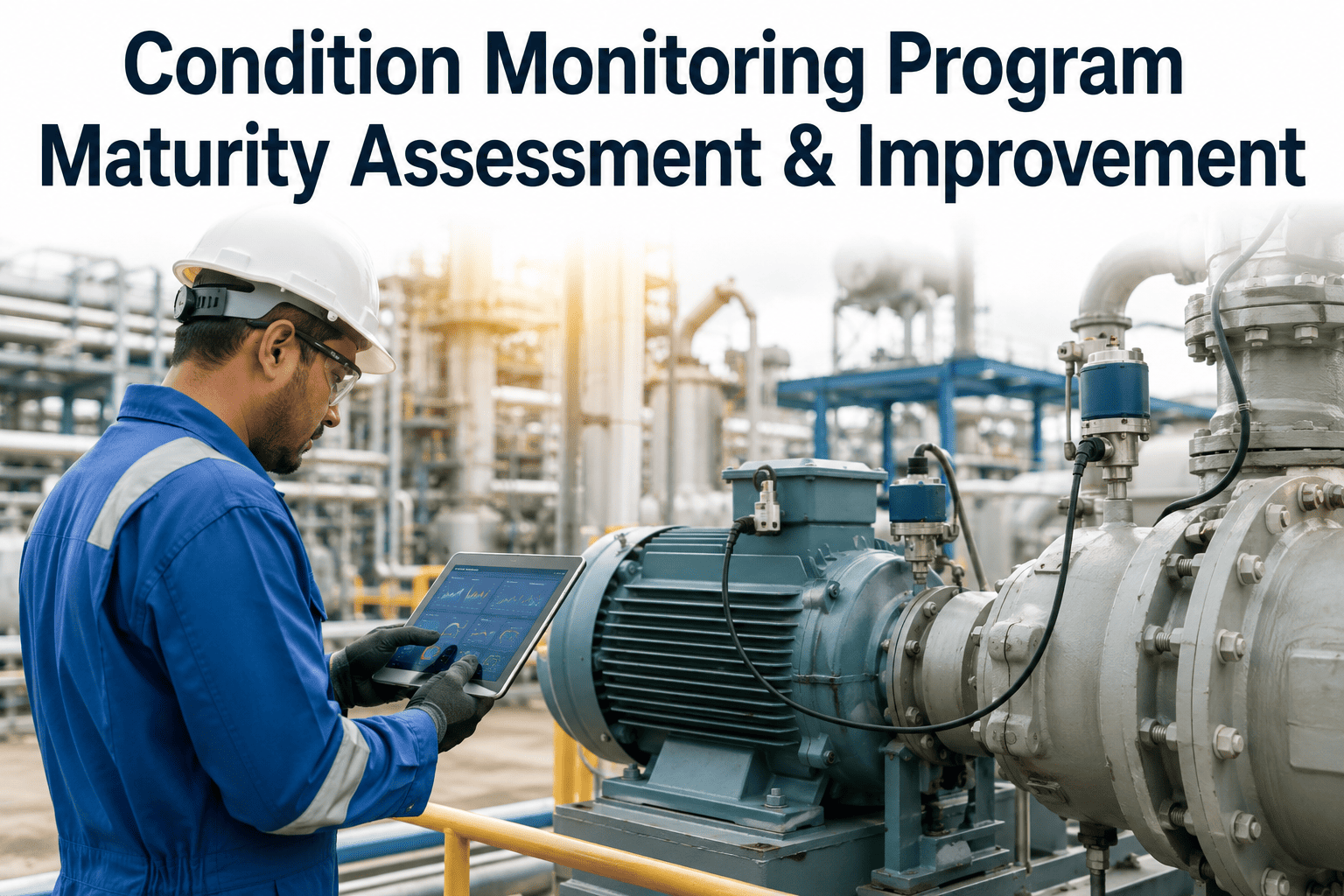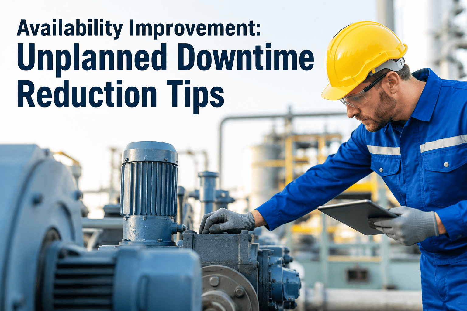
Most plants can tell you what broke last week. Almost none can tell you where the other 20-30% of their production capacity silently disappeared this quarter. That gap between what a line could produce and what it actually produces lives inside a single OEE component: Availability. When Availability drags OEE down, the plant is not slow and it is not making bad parts — it simply is not running when it is supposed to be running. iFactory's downtime and reliability intelligence platform closes that gap by connecting root cause elimination, PM optimization, and condition monitoring into one system instead of three disconnected initiatives.
Low OEE Almost Always Starts With Availability, Not Speed or Quality
Availability is the first of the three OEE multipliers, and it is usually the biggest lever. A plant losing 30% of its scheduled time to unplanned downtime cannot out-run or out-quality its way back to world-class OEE. It has to fix Availability first.
Why Availability Loss Is Different From Performance or Quality Loss
Performance loss and quality loss are visible while the line is running — a slow cycle, a scrapped part. Availability loss is invisible until you go looking for it, because it lives in the gaps between production runs: the breakdown at 2 a.m. that nobody logged with a real reason code, the changeover that took forty minutes because a fixture was missing, the small stop that never made it into a report because the operator restarted the line in ninety seconds. Individually these look like noise. Aggregated across a month, they are usually the single largest block of lost capacity on the floor.
The Six Big Losses framework, developed as part of Total Productive Maintenance, assigns every one of these events to a category so that engineering teams stop treating a bearing failure and a changeover delay as the same problem requiring the same fix. Availability loss splits into exactly two buckets:
This article focuses on the unplanned side, because it is where the largest and least understood losses live, and because it responds directly to three specific, well-documented interventions: root cause elimination, PM optimization, and condition monitoring.
It also matters because unplanned downtime is disproportionately expensive relative to how it looks on a shift report. A forty-minute changeover shows up as forty minutes of lost run time and nothing else. A forty-minute unplanned stop shows up as forty minutes of lost run time plus emergency labor pulled off other work, plus a rush order for a part that would have cost less on standard lead time, plus every downstream operation that was scheduled to run behind the failed asset now sitting idle too. Industry cost-per-hour figures for unplanned downtime commonly range from the low tens of thousands of dollars for a mid-size plant to several hundred thousand dollars per hour in high-throughput or high-value production, and those figures typically capture only the direct production loss — not the schedule recovery cost that follows.
That asymmetry is exactly why Availability deserves to be the first target when OEE is low. A plant that improves Performance by five points but is still losing three hours a week to unplanned breakdowns has fixed the smaller problem. Availability gains compound in a way Performance gains often do not, because every hour of unplanned downtime eliminated is an hour that becomes available for either more good production or a properly scheduled PM window — which in turn reduces the next unplanned stop.
See Your Actual Availability Loss, Broken Down by Cause
iFactory logs every stop with a structured reason code automatically, so your team stops guessing which loss category is costing the most and starts fixing the one that actually is.
The Three Levers That Actually Move Availability
Plants that move from average OEE (55-65%) to top-quartile OEE (80%+) almost never do it through a single silver-bullet initiative. They pull three specific levers, usually in this order, because each one builds the data foundation the next one needs.
Root Cause Elimination
Stop replacing the failed part and start asking why it failed. Root Cause Failure Analysis (RCFA) traces a breakdown back through the physical, human, and process layers — a seized bearing might trace back to a lubrication interval that was never adjusted for actual load, not a bad batch of grease.
PM Optimization
Calendar-based preventive maintenance treats every asset the same regardless of actual duty cycle, which means healthy equipment gets over-serviced while hard-running equipment fails between scheduled visits. PM optimization rebuilds intervals around failure mode data, criticality, and — where available — runtime hours rather than a fixed calendar date.
Condition Monitoring
Vibration, thermal, and current signature monitoring catch degradation while it is still a trend line, not yet an alarm. This is what lets a plant intervene during a planned window instead of an emergency one — the single biggest driver of the cost gap between predictive and reactive maintenance.
Sequencing the Three Levers: A Practical Rollout
Plants that try to run all three levers simultaneously from a standing start usually stall out, because condition monitoring is only useful once you know which assets are worth instrumenting, and PM optimization only works once you have real failure mode data to optimize against. The practical sequence looks like this:
| Phase | Primary Lever | What Happens | Typical Duration | iFactory Role |
|---|---|---|---|---|
| Phase 1 | Root Cause Elimination | Every unplanned stop gets a structured reason code and, above a defined cost threshold, a formal RCFA. Bad actors identified via Pareto ranking. | 4-8 weeks | Automated downtime logging + reason code taxonomy |
| Phase 2 | PM Optimization | PM schedules rebuilt using the failure modes surfaced in Phase 1 — intervals extended on over-serviced assets, tightened on under-serviced ones. | 6-10 weeks | Failure-mode-linked PM template library |
| Phase 3 | Condition Monitoring | Sensors deployed on the highest-criticality assets identified in Phases 1-2. Alerts routed to the same work order system as PM and reactive work. | 8-12 weeks | Real-time anomaly alerts tied to auto-generated work orders |
| Phase 4 | Continuous Loop | Every new failure feeds back into the RCFA process, every RCFA output feeds back into PM intervals, and monitoring thresholds are recalibrated quarterly. | Ongoing | Closed-loop analytics dashboard across all three levers |
Sequencing This Correctly Is the Difference Between a 90-Day Win and a Stalled Initiative
iFactory's implementation team helps you identify which assets belong in Phase 1 versus Phase 3, so condition monitoring dollars go to the equipment that actually needs them.
What Root Cause Elimination Looks Like in Practice
Root cause elimination is often confused with troubleshooting, but the two produce different outcomes. Troubleshooting answers "how do we get the line running again" and typically ends with a replaced part. Root cause failure analysis answers "why did this specific failure mode occur, and what condition allowed it to happen" — and it does not stop until the answer is something the plant can actually correct, not just something that happened to be true.
A useful way to think about it: every failure has a physical root cause, a human root cause, and often a latent system root cause. A bearing seizes (physical). The technician who last serviced it had not been trained on the updated lubrication spec for that duty cycle (human). The PM procedure documentation was never updated when the asset was moved to three-shift operation eighteen months earlier (latent/system). Stopping at "replace the bearing" fixes nothing. Stopping at "retrain the technician" fixes the human layer but leaves the outdated procedure in place for the next technician. Only closing all three layers actually eliminates the failure mode.
Not every failure warrants this level of investigation — a full RCFA can consume eight to sixteen hours of combined engineering and maintenance time. The discipline is in setting a clear threshold: failures above a defined cost, safety severity, or repeat-occurrence count trigger a full RCFA; everything else gets a fast structured method such as 5-Why, still documented, still feeding the same reason-code database, just without the multi-day investigation. Plants that skip this threshold either burn out their reliability engineers running full RCFA on every minor stop, or never run it at all because nobody has time — both outcomes stall Availability improvement at the same point.
Prioritizing Which Loss to Attack First
Not every line, cell, or asset deserves the same level of intervention. The Pareto principle applies directly here: identify the single largest availability loss category on a given line, focus improvement resources there until it stabilizes, and only then move to the next category. Spreading effort evenly across every asset in the plant produces slower results than concentrating on the top two or three bad actors.
Why Calendar-Based PM Alone Cannot Close the Gap
Calendar-based preventive maintenance is built on an assumption that does not hold up well under scrutiny: that failure probability rises predictably with time or usage, so servicing everything on a fixed schedule prevents most failures. Research into failure conditional-probability patterns across complex equipment consistently finds that a large majority of failures do not follow a simple wear-out curve tied to age. Some failure modes are genuinely random with respect to time in service, some show early "infant mortality" shortly after a component is installed or serviced, and only a minority show the traditional bathtub-curve wear-out pattern that calendar-based PM is designed around.
The practical consequence is that a fixed interval is wrong for most of the assets it is applied to. On assets with a random failure pattern, calendar PM performs unnecessary work with no measurable effect on failure rate — the equivalent of changing your oil every three months regardless of miles driven. On assets running harder than the interval assumes, calendar PM misses the failure entirely, because the equipment reaches its actual wear limit before the next scheduled service. This is the exact scenario reliability teams see repeatedly: a critical asset running three shifts fails between PM visits designed for a single-shift duty cycle, while a lightly used sister asset on the same interval gets serviced with plenty of useful life still remaining in its components.
PM optimization does not mean abandoning scheduled maintenance. It means rebuilding the interval logic around actual failure mode data — informed by RCFA findings, by runtime or cycle-count data where available, and by criticality ranking — rather than a single calendar assumption applied uniformly across dissimilar assets.
Common Mistakes That Keep Availability Flat
Logging downtime without structured reason codes. A stop labeled "machine down" tells you nothing a Pareto analysis can act on. Every stop needs a cause category, an asset ID, and a duration captured automatically — not reconstructed from memory at end of shift.
Running RCFA on every failure, or none of them. Full RCFA is expensive in engineering time. Set a clear cost or safety threshold for which failures trigger a full investigation, and use fast 5-Why for the rest.
Buying sensors before fixing the PM program. Condition monitoring on an asset with an already-broken maintenance process just adds another alert nobody acts on. Fix the workflow first, then instrument it.
Treating calendar-based PM as equivalent to condition-based PM. Research on failure patterns shows the large majority of failures are not simply age-related, which means a fixed calendar interval will always either over- or under-maintain a meaningful share of the asset base.
Availability Improvement KPIs to Track
Availability Rate
Run Time divided by Planned Production Time. The foundational OEE input and the clearest single measure of whether these three levers are working.
Reactive Work Percentage
Share of total maintenance hours spent on unplanned, emergency work. A falling trend is the clearest early signal that root cause elimination and PM optimization are taking hold.
PM Compliance
Percentage of scheduled preventive maintenance completed within its defined window. Low compliance quietly erodes every other Availability gain.
Repeat Failure Rate
Same asset, same failure mode, within a rolling 90-day window. This is the single best proxy for whether RCFA findings are actually being implemented, not just documented.
Mean Time Between Failures
Average operating time between breakdowns on a given asset class. Should trend upward consistently as condition monitoring coverage expands.
Mean Time to Repair
Average time from stop to restart. Improves as reason codes get more precise and technicians arrive with the right parts and procedure already known.
The plants that struggle with Availability are almost never short on maintenance effort. They are short on sequencing. I have walked into facilities running world-class vibration monitoring on an asset that still has a calendar-based PM plan nobody has touched in six years, and reactive work orders for the exact same bearing failure four times in one year with no RCFA ever opened. The fix is rarely more technology. It is closing the loop between what a failure teaches you and what your PM plan and your monitoring thresholds actually do about it.
Frequently Asked Questions
World-class Availability generally sits above 90%, which combined with Performance and Quality targets produces the commonly cited 85%+ world-class OEE benchmark. Most discrete manufacturing plants operate with Availability closer to 75-85%, and plants still relying heavily on reactive maintenance often see 60-70%. The right target depends on your industry and equipment criticality — a semiconductor fab and a food packaging line have very different acceptable downtime profiles. iFactory's benchmarking tools can show how your Availability compares against your own historical baseline, which is usually more actionable than a generic industry number.
Start with root cause elimination. It requires the least upfront investment, generates the failure mode data that makes PM optimization accurate, and identifies which assets are actually worth a condition monitoring investment. Plants that reverse this order — buying sensors before fixing the underlying maintenance process — typically see disappointing ROI because the alerts have nowhere productive to go. Run all three in a continuous loop once the initial sequence is established, rather than treating any of them as a one-time project.
Documented industry results for predictive and structured preventive maintenance programs generally fall in the 30-50% unplanned downtime reduction range versus a purely reactive baseline, though results vary significantly by starting condition and asset mix. Plants starting from a low base — heavy reactive maintenance, no structured reason codes — tend to see the largest early gains because the lowest-hanging fruit is still on the tree. Book a demo to walk through what a realistic first-year target looks like for your specific asset base.
No — root cause elimination and PM optimization alone typically recover a meaningful share of lost Availability without any new hardware, because most of that loss comes from process gaps, not a lack of sensor data. Condition monitoring adds real value on high-criticality, high-cost assets where gradual degradation patterns exist, but it is the third lever, not the first. Many plants get 12-24 months of solid Availability gains before condition monitoring hardware becomes the highest-ROI next investment.
Availability loss means the equipment was scheduled to run and was not running at all — a full stop, whether planned (changeover) or unplanned (breakdown). Performance loss means the equipment was running but below its rated speed, through small stops or slow cycles. The two require different fixes: Availability responds to reliability engineering and maintenance strategy, while Performance typically responds to operator training, process tuning, and equipment condition affecting cycle speed. iFactory's OEE dashboard separates the two automatically so improvement teams are not solving a Performance problem with an Availability-focused fix.
Turn Three Disconnected Initiatives Into One Availability System
iFactory connects downtime logging, root cause tracking, PM scheduling, and condition monitoring alerts into a single platform — so every failure makes the next PM cycle smarter and every PM cycle makes the next monitoring threshold more accurate.