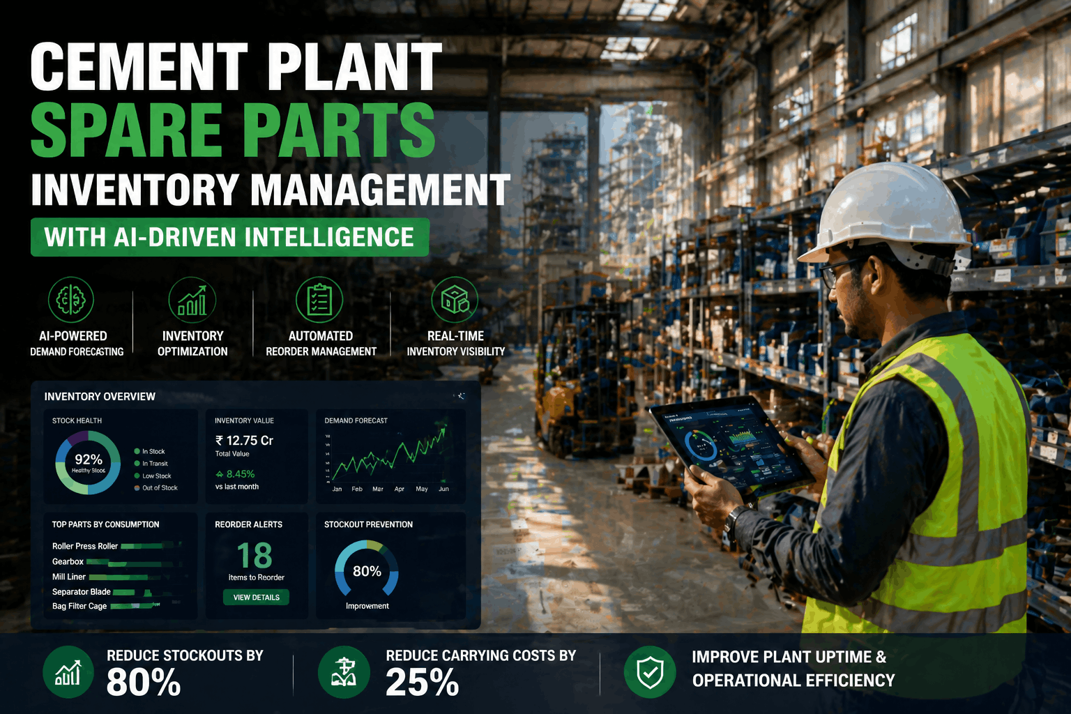
A cement plant warehouse that looks well-stocked is often hiding a problem that only surfaces when the finance team runs the annual inventory carrying cost report. Shelves are full, but 20 to 30 percent of the parts on those shelves have not moved in two or more years. Meanwhile, a critical gearbox component with a twelve-week lead time just ran out of stock because the reorder point was set based on average monthly consumption that did not account for the preventive maintenance schedule that drives 80 percent of the actual demand. The result is a warehouse that is simultaneously overstocked and understocked, tying up capital in dead inventory while failing to protect production from the specific stockouts that cause the most damage. iFactory's inventory management platform applies AI consumption analytics to this exact problem, forecasting demand from the maintenance patterns that actually drive parts usage rather than the crude historical averages that miss them.
Your warehouse is full but your production line is still waiting for parts
AI-driven spare parts consumption analytics replaces guesswork and historical averages with demand forecasts tied to actual maintenance schedules, equipment condition data, and operating patterns, typically reducing inventory carrying costs by 15 to 25 percent while cutting stockout-related downtime by over half.
Why cement plants are uniquely vulnerable to inventory failure
Spare parts management in a cement plant bears almost no resemblance to spare parts management in a discrete manufacturing facility. A car plant consumes thousands of SKUs in predictable quantities tied to production volume. A cement plant consumes a smaller number of highly specialized SKUs in quantities that have almost no correlation to production volume because consumption is driven almost entirely by maintenance events, not throughput. A raw mill that runs 7,500 hours in a year might consume zero grinding elements if the maintenance team replaced them just before the year started, or it might consume two full sets if an unexpected material change accelerated wear. The same production output, completely different parts consumption.
This disconnect between production volume and parts demand is the root cause of the inventory paradox that plagues nearly every cement plant warehouse. Procurement teams, lacking a better signal, set reorder points and safety stock levels based on historical consumption averaged across long time periods. This averaging works reasonably well for high-volume consumables like lubricants, filters, and conveyor belts that are used continuously. But it fails completely for the components that matter most, the medium and low-volume parts whose consumption is episodic, driven by specific maintenance tasks, and highly sensitive to the timing of those tasks relative to the reorder cycle.
The practical consequence is a warehouse that performs poorly on both sides of its core function. Critical parts stock out because their consumption spike was smoothed away by the averaging process, and non-critical parts accumulate because their reorder points were set too high by the same averaging process that missed the spike on the other end. The warehouse looks busy and full, but it is not doing the one thing it exists to do, which is ensuring that the right part is available at the right time without carrying more inventory than necessary to achieve that objective.
Four forecasting methods and the specific ways they break down in cement
Most cement plants use one or more of four traditional forecasting approaches, each of which was designed for environments where demand is relatively steady and consumption correlates with production volume. None of them were designed for an environment where a single scheduled maintenance event can generate more parts demand in one week than the previous six months combined. Understanding exactly how each method fails is important because it explains why simply switching from one traditional method to another does not solve the problem. The failure is structural, not procedural.
Reorder point methods fail because they treat demand as a continuous flow when it is actually a series of discrete events. A kiln section might consume zero refractory anchor bolts for eleven months and then consume 400 of them during a two-week shutdown. A reorder point calculated from monthly averages will either trigger too early, generating excess inventory that sits for months, or too late, triggering an emergency order that arrives after the shutdown window has closed. The method cannot distinguish between steady consumption and burst consumption because it has no visibility into why the consumption happens.
Min/max methods add a ceiling to the reorder point approach but inherit the same fundamental weakness. The maximum level is typically set based on the largest historical consumption quantity in a given period, which means a single unusually large order, perhaps caused by a one-time failure rather than scheduled maintenance, permanently inflates the max level for that SKU. Over time, max levels drift upward and never come back down because there is no mechanism to distinguish between repeatable demand and one-time anomalies.
ABC analysis categorizes parts by spend volume but tells you nothing about when those parts will be needed. A Class A part that accounts for 15 percent of total inventory spend might be needed once every two years during a major overhaul, while a Class C part that accounts for 1 percent of spend might be needed every three weeks. ABC analysis correctly identifies that the Class A part deserves more procurement attention, but it provides no guidance on when to order it, how much safety stock to hold, or how to align the order with the overhaul schedule. It is a prioritization tool, not a forecasting tool, and cement plants that rely on it as their primary inventory management method are essentially using a categorization system to solve a timing problem.
Subjective judgment, where an experienced storekeeper or maintenance planner sets reorder points based on personal experience, is the most flexible of the four methods but also the most fragile. It works well as long as the person with the experience is present, but that knowledge walks out the door every time a senior planner retires or transfers. It also scales poorly, as no individual can maintain accurate mental models of demand patterns for more than a few hundred SKUs, and cement plant warehouses typically hold 3,000 to 8,000 active SKUs.
From raw transaction data to a living demand forecast
AI consumption analytics works differently from traditional methods because it does not assume that past consumption is a stable predictor of future consumption. Instead, it treats parts consumption as a dependent variable that is influenced by multiple upstream factors, some of which are observable and some of which can be inferred from patterns in the data. The model's job is not to extrapolate a trend line from historical usage but to identify the causal relationships between maintenance activities, equipment condition, operating parameters, and the resulting parts consumption, then use those relationships to forecast what will be needed next.
Historical Ingestion
Parts issuance transactions, work order histories, and purchase orders are loaded into the model to establish baseline consumption patterns per SKU.
PM Correlation
The model maps which parts are consumed by which preventive maintenance tasks, creating a direct link between the maintenance schedule and parts demand.
Pattern Learning
Machine learning identifies recurring consumption patterns, seasonal shifts, and correlations with operating hours or production campaigns that human analysis misses.
Demand Forecasting
For each SKU, the model generates a rolling demand forecast that accounts for upcoming PM tasks, known equipment condition, and lead time requirements.
Reorder Optimization
Dynamic reorder points and safety stock levels are calculated and updated automatically, replacing static thresholds with values that reflect current conditions.
The PM correlation step is where AI delivers the most value over traditional methods. When the model learns that a specific set of seals, bearings, and liners is consistently consumed during the raw mill quarterly PM, it can forecast that demand with high confidence because it knows the PM is scheduled. It does not need to wait for the consumption to happen and then react to it. It anticipates it, checks current stock levels against the forecasted demand plus lead time, and generates a procurement recommendation with enough lead time for the parts to arrive before the PM window opens. This is fundamentally different from a reorder point system that only triggers after stock has already fallen below a threshold, which often means the trigger fires too late for parts with long lead times.
The pattern learning step catches the consumption drivers that are not directly tied to scheduled maintenance. A cement plant might observe that grinding media consumption in the cement mill increases by 20 to 30 percent during periods when the clinker is harder, which correlates with specific quarry faces being active. A human planner might notice this pattern intuitively but cannot systematically apply it to procurement timing for hundreds of SKUs. The model detects it automatically and adjusts the forecast for grinding media, and any other parts whose consumption correlates with the same operating parameter, without being explicitly told to look for that specific relationship.
What the model needs and how each source contributes
The accuracy of an AI consumption forecast is directly proportional to the quality and breadth of the data feeding it. A model that only has parts issuance history can still outperform traditional methods because it can detect patterns and seasonality that averaging misses. But a model that also has maintenance schedules, equipment condition data, and operating parameters can achieve a level of forecasting accuracy that transforms the warehouse from a cost center into a production enabler. The data inputs below are ranked by their contribution to forecast accuracy in a typical cement plant environment, based on implementations across multiple sites.
Parts Issuance History
The foundational data source. Every transaction recording when a part was issued, which equipment it was used on, and which work order it was associated with. Minimum 18 to 24 months of clean transaction data is needed to establish reliable baseline patterns for most SKUs.
Preventive Maintenance Schedule
The forward-looking demand driver. When the model knows which PM tasks are scheduled for the next three to six months and which parts those tasks typically consume, it can forecast demand with high confidence before any consumption actually occurs.
Equipment Condition Data
Vibration trends, temperature readings, and oil analysis results that indicate whether equipment is degrading faster or slower than expected. Degrading equipment accelerates parts consumption, and the model adjusts forecasts upward accordingly.
Operating Hours and Production Data
Cumulative operating hours per equipment and production throughput data that serve as leading indicators for wear-dependent parts. More operating hours in a given period means more wear, which means more parts consumption is coming.
Supplier lead time data is a secondary but important input that affects the reorder point calculation more than the demand forecast itself. A part with a four-week lead time requires a different procurement trigger than the same part with a twelve-week lead time, even if the demand forecast is identical. The model uses historical purchase order data to calculate actual lead time variability, not just the supplier's quoted lead time, because the quoted number often understates the real experience by 30 to 50 percent. This variability calculation is what determines the safety stock level, which is the buffer that protects against the gap between expected and actual lead time.
See what AI consumption analytics would find in your warehouse data
iFactory ingests your parts issuance and maintenance history to build a demand forecast model customized to your plant, showing exactly where traditional methods are over-ordering and under-ordering.
Where the excess inventory actually comes from
When a cement plant conducts its first rigorous inventory audit after implementing AI consumption analytics, the dead stock breakdown almost always follows a similar pattern. The percentages vary by plant, but the categories are remarkably consistent because the root causes are structural to how cement plants have traditionally managed their warehouses. Understanding these categories matters because each one has a different prevention strategy, and treating them all as generic "excess inventory" misses the opportunity to prevent the specific behavior that created each category.
Obsolete equipment parts represent the largest dead stock category in most cement plants because equipment replacement or modification projects often leave behind a inventory of spare parts for the old configuration. A baghouse upgrade might change the filter bag dimensions, rendering the existing filter bag inventory obsolete, but those old bags remain in the warehouse because nobody has gone through the formal disposition process to write them off. Over a plant's operating life, these accumulation events compound, and the result is shelves full of parts that will never be used but are still being counted in the inventory valuation and incurring carrying costs.
Over-ordering from poor forecasting is the category that AI consumption analytics attacks most directly. When reorder points are set too high because the forecasting method cannot distinguish between one-time demand and repeatable demand, every reorder cycle generates a small surplus that accumulates over time. A part that is actually consumed once per quarter but whose reorder point assumes monthly consumption will accumulate three months of excess stock per year. Multiply that dynamic across hundreds of SKUs and the dollar value of the surplus becomes significant very quickly. AI forecasting eliminates this by tying the reorder trigger to the actual demand driver, the maintenance schedule, rather than a smoothed average that overestimates steady-state consumption.
Duplicate SKUs accumulate over years of procurement without standardized part numbering. The same bearing might exist in the system under three different part numbers because three different planners ordered it from three different suppliers over a decade. Each number has its own reorder point and safety stock, so the plant is effectively holding three times the necessary inventory for that single physical part. AI analytics helps identify these duplicates by analyzing consumption patterns across SKUs and flagging items with highly correlated issuance timing and quantities, which often indicates they are the same part under different numbers.
How demand predictions become warehouse actions
A demand forecast that stays in a report is worthless. The entire value of AI consumption analytics is realized only when the forecast drives actual procurement decisions in a way that is faster, more accurate, and more consistent than what a human planner can achieve manually. The translation from forecast to action requires a structured process that connects the model's output to the procurement workflow without creating a parallel system that operators and planners have to maintain separately from their existing tools.
Dynamic Reorder Point Calculation
The model recalculates reorder points for every active SKU on a weekly or biweekly cadence, replacing static thresholds with values that reflect the current demand forecast, upcoming PM tasks, and actual supplier lead time performance. Reorder points that were set once during system implementation and never touched again are replaced by living values that adapt to changing conditions.
Automated Procurement Triggers
When current stock plus on-order quantity falls below the dynamic reorder point, a purchase recommendation is generated automatically with the suggested order quantity, preferred supplier, and required delivery date. The procurement team reviews and approves rather than initiating from scratch, which reduces the cycle time from identification to PO by days.
Safety Stock Recalibration
Safety stock levels are continuously adjusted based on observed lead time variability and demand forecast error. Parts with highly predictable demand and reliable suppliers get reduced safety stock, freeing working capital. Parts with erratic demand or unreliable suppliers get increased safety stock to protect against the specific risks they face.
PM-Aligned Purchasing
For parts whose demand is driven by known PM tasks, the system generates purchase recommendations timed to ensure arrival before the scheduled PM window. This eliminates the common situation where a PM task is delayed because parts were not ordered early enough, which is one of the most frequent causes of PM compliance degradation in cement plants.
The cumulative effect of these four actions is a warehouse that operates proactively rather than reactively. Instead of discovering during a PM kickoff that a critical seal is out of stock and then scrambling to find it from another plant or an expensive local supplier, the procurement team receives the order recommendation six to eight weeks before the PM is scheduled, reviews it in the context of their current supplier agreements, and places the order with comfortable lead time. The maintenance team gets its parts on time, the procurement team avoids premium pricing, and the warehouse carries exactly what it needs for the upcoming demand window without excess.
Planners who have worked with AI-driven procurement recommendations consistently report that the biggest behavioral change is not the automation itself but the shift from reactive to forward-looking work. When reorder points are static, the planner's day is dominated by expediting late orders and resolving stockouts. When reorder points are dynamic and PM-aligned, the planner's day shifts to reviewing upcoming demand windows, validating model recommendations, and optimizing supplier agreements, which is higher-value work that directly improves plant reliability.
What cement plants report after implementing AI consumption analytics
The financial and operational impact of AI-driven spare parts management in cement plants follows a predictable pattern across implementations. The first 60 days are dominated by data cleanup and baseline establishment, which often surfaces immediate savings from duplicate SKU consolidation and obvious overstock situations. The 60 to 180 day window is where the demand forecast models mature and dynamic reorder points begin replacing static ones, producing measurable reductions in both stockout events and inventory value. Beyond 180 days, the compounding benefits of continuous model learning and PM-aligned procurement become visible in the metrics that plant managers and finance teams track most closely.
Beyond these direct metrics, the most frequently cited benefit is one that does not appear on any standard inventory report: the elimination of the emergency procurement scramble. Maintenance planners and procurement teams in cement plants that have implemented AI consumption analytics describe a qualitative shift in their daily work that is difficult to quantify but immediately noticeable. The phone calls from the maintenance floor asking whether a part is in stock, the urgent requests to source a component from a competitor plant, the premium freight charges for parts that should have been ordered weeks ago, these events do not disappear entirely but they become rare exceptions rather than routine occurrences. For teams that have spent years operating in reactive mode, this shift in daily experience is often more impactful than the inventory value reduction that shows up on the balance sheet.
The carrying cost savings alone typically justify the investment within the first year. A mid-size cement plant carrying $4 million in spare parts inventory at a 25 percent annual carrying cost is spending $1 million per year just to hold that inventory. A 22 percent reduction in inventory value translates to $220,000 in annual carrying cost savings, plus the avoided costs of emergency procurement, premium freight, and delayed maintenance that are no longer occurring. For large integrated cement plants with multiple production lines and warehouse values exceeding $10 million, the savings scale proportionally and often reach seven figures within the first 18 months.
Spare parts consumption analytics, explained plainly
Stop guessing what your warehouse needs. Start knowing.
iFactory ingests your cement plant's parts data, maps it to your maintenance schedule, and delivers AI-driven demand forecasts that reduce inventory costs while eliminating the stockouts that stop production.