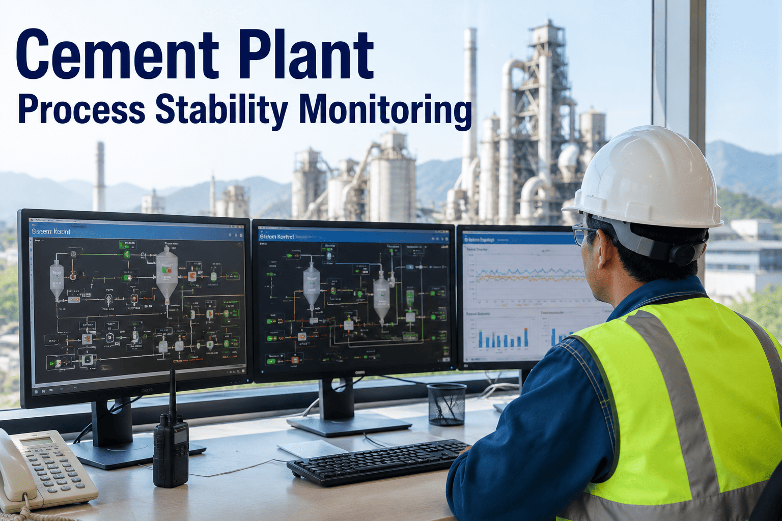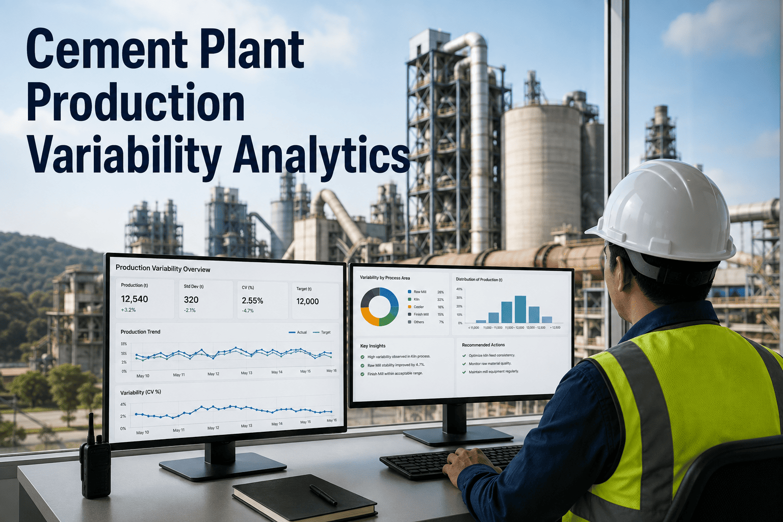
A cement plant that hits its average monthly production target can still be losing significant margin if that average is masking wide swings between good days and bad days. A kiln that runs smoothly for three weeks and then stumbles through five days of feed instability, temperature hunting, and quality rework often produces the same monthly tonnage as a kiln that ran consistently the entire time, but at a meaningfully higher energy and labor cost. Book a demo to see how variability analytics exposes the difference.
Your Monthly Average Is Hiding the Real Story of How Your Plant Runs
iFactory tracks process stability across your cement plant in real time, surfacing the swings, drifts, and instability windows that a monthly production summary smooths over completely.
Two Plants With the Same Monthly Output Can Have Very Different Cost Structures
Monthly production reports are built around totals and averages, tons produced, average energy per ton, average downtime hours, because those are the numbers that roll up cleanly into a summary. What that summary hides is the shape of the month underneath it. A plant that runs at a consistent, well-controlled setpoint every single day will generally consume less energy per ton, produce more consistent clinker quality, and put less wear on equipment than a plant that swings between overcorrected high-feed periods and underfed low-output periods, even if both plants finish the month with the same total tonnage.
Variability itself has a cost, separate from downtime and separate from average output. Every time a process parameter drifts outside its stable range and has to be corrected, that correction consumes energy, stresses equipment, and increases the chance of an off-spec batch reaching quality control. A plant serious about reducing operating cost has to look past the monthly average and start measuring how stable the process actually was, day by day and shift by shift.
This gap between averages and reality is why two plants producing what appears to be an identical product at an identical volume can have meaningfully different profitability. The plant running a tighter, more stable process spends less on energy correcting for swings, sends fewer batches back for rework, and puts less cumulative stress on equipment that has to absorb the physical strain of repeated large corrections. None of that shows up clearly in a monthly summary built around totals, which is exactly why so many plants underinvest in stability monitoring even when the underlying cost is real and ongoing.
Six Common Sources of Production Variability in a Cement Plant
Instability rarely traces back to a single cause. More often it is a combination of two or three of the following factors compounding on each other, which is exactly why a targeted, data-driven diagnosis matters more than a generic corrective action applied across the board.
What Process Stability Monitoring Actually Tracks
Stability monitoring is not simply another set of numbers layered on top of the standard production report. Each of the following metrics answers a different question about how the process behaves between the moments a deviation begins and the moment it gets corrected, which is precisely the window that a monthly total never captures.
| Metric | What It Reveals |
|---|---|
| Setpoint deviation frequency | How often a parameter drifts outside its stable operating band |
| Time to correction | How quickly a deviation gets identified and corrected once it begins |
| Correction magnitude | Whether operators are making small adjustments or large, destabilizing corrections |
| Shift-to-shift variance | Whether process stability differs meaningfully depending on who is operating |
| Recovery time after disruption | How long it takes the process to return to stable operation after an upstream event |
iFactory tracks setpoint deviation, correction patterns, and recovery time across every shift so instability gets caught and addressed instead of averaged away in the monthly report.
A Four-Step Approach to Reducing Process Variability
Reducing variability works best as a structured, repeatable cycle rather than a one-time push, since new sources of instability can appear as equipment ages, raw material sources change, or staffing shifts. The four steps below give a plant a consistent way to work through the problem, whether it is being applied for the first time or repeated as part of an ongoing improvement rhythm.
What Changes When a Plant Moves From Reactive to Monitored Stability
The shift from an unmonitored to a monitored process is less about installing new sensors and more about changing what the plant pays attention to on a daily basis. The comparison below reflects the practical differences plants typically describe once stability metrics become part of the regular operating rhythm rather than an occasional special study.
| Dimension | Unmonitored Process | Monitored Process |
|---|---|---|
| Deviation detection | Noticed after quality or output impact | Flagged as soon as it begins drifting |
| Shift consistency | Varies widely by operator judgment | Guided by shared, data-backed response standards |
| Energy consumption | Elevated by frequent large corrections | Reduced through smaller, earlier corrections |
| Quality rework | Reactive, discovered at lab testing | Reduced through tighter process control |
What Reduced Variability Typically Delivers Within a Quarter
These outcomes compound on each other rather than arriving independently. Lower energy consumption and reduced rework both flow from the same underlying improvement, a process that spends more time near its stable setpoint and less time recovering from large, avoidable swings.
Common Questions About Production Variability Analytics
Isn't some process variability just unavoidable in cement production?
Some variability is genuinely unavoidable, raw material composition will never be perfectly uniform and equipment will never respond with zero lag, but the goal of variability analytics is not to eliminate every fluctuation, it is to distinguish between normal, expected variation and abnormal instability that signals a correctable problem. A well-controlled process still has some noise around its setpoints, but that noise stays within a predictable, tight band. What variability analytics catches is the difference between that normal band and the wider swings that come from an unaddressed root cause, which is where the real cost and quality impact actually lives. Book a demo to see what your normal variability band looks like today.
How does this differ from the alarms already built into our DCS system?
A DCS alarm typically triggers when a parameter crosses a hard threshold, which catches acute deviations but misses the slower, cumulative pattern of instability that never quite trips an alarm yet still drives up energy consumption and quality variance over time. Variability analytics looks at the shape of process behavior over hours and shifts rather than a single threshold crossing, surfacing patterns like a parameter that oscillates more widely than it used to, or a shift that consistently takes longer to correct deviations than other shifts. These patterns are invisible to a standard alarm system because no individual reading ever crosses the alarm limit.
Can this identify whether a specific shift or operator is contributing to instability?
Yes, shift-level comparison is one of the more actionable outputs, though it works best when framed as a coaching and standardization opportunity rather than a disciplinary one. Differences between shifts usually reflect differences in training, experience, or informal technique rather than effort, and surfacing the data typically leads to the most stable shift's approach being documented and shared as the standard response for common deviations. Plants that use this data constructively tend to see the gap between their most and least stable shifts narrow significantly within a few months as best practices spread across the team.
Does reducing variability require new equipment or automation upgrades?
Not necessarily. A significant portion of process variability in most plants comes from inconsistent human response to deviations rather than equipment limitations, which means standardizing correction procedures and giving operators earlier visibility into forming deviations can produce meaningful improvement without any capital investment. In cases where equipment condition drift, such as a wearing valve or a degrading sensor, is identified as a root cause, that specific piece of equipment may warrant investment, but the broader variability reduction program is primarily about process discipline and earlier detection rather than automation. Contact support to discuss what a variability reduction program looks like for your plant.
How long does it take to see measurable improvement after starting to monitor variability?
Most plants establish a reliable baseline within the first month of monitoring, since that requires enough shift cycles to distinguish normal variation from genuine instability patterns. Once root causes are identified and standardized response procedures are put in place, measurable improvement in energy consumption and quality consistency typically becomes visible within the following one to two months, though the full benefit compounds over a longer period as the new procedures become habitual across every shift. Plants that treat this as a one-time project rather than an ongoing monitoring practice tend to see gains erode within a year as old habits and undetected drift creep back in. Book a demo to build a monitoring plan suited to your production schedule.
Stop Letting the Monthly Average Hide Where Your Real Costs Live
iFactory surfaces the day-to-day and shift-to-shift instability driving your energy and quality costs, so your team can standardize what's already working and correct what isn't.