Every cement plant lab generates thousands of data points a week — free lime, LSF, SM, AM, Blaine fineness, 1-day strength, 3-day strength, 28-day strength, insoluble residue, sulfate, chloride, alkali, loss on ignition — and in most plants that data ends up in a spreadsheet nobody opens between month-end reports. The lab did the work. The results are technically "in the system." But the trend that would have caught the free lime drift three days before the specification breach, the correlation between raw mix chemistry and 1-day strength that would have predicted the Monday delivery problem, the process capability index that would have shown the 43-grade cement running at Cpk 0.8 for six weeks — none of that surfaces from the underlying data because nothing is turning the data into analysis. LIMS data analytics closes that gap by putting the trending, correlation, and prediction layer on top of the results the lab is already producing. Cement quality teams evaluating this can Book a Demo to see how iFactory turns cement LIMS data into proactive quality intelligence.
The Gap Between "We Have LIMS" and "We Have LIMS Analytics"
Most cement plants passed the "we have LIMS" milestone years ago. Samples get logged, tests get scheduled, results get entered, certificates of analysis get generated. That is table stakes and it is genuinely useful — the paper binder era is over and nobody wants it back. But structured storage of results is not analytics. Analytics is what happens when the results become the input to trending charts, correlation studies, and prediction models that turn historical data into forward-looking intelligence. The gap between the two is where most cement quality programs still operate: results are captured cleanly, but the analysis that would make the results actionable in the next shift instead of the next month is not happening.
The evidence of the gap is easy to spot. Quality parameters trend out of specification and nobody knew until the batch shipped. Free lime drifts upward for a week and nobody investigated the cause because nobody was watching the trend line. Raw mix chemistry changes as the quarry face moves and finished cement strength drops two weeks later without anyone connecting the two events. A 28-day strength number arrives showing the material was under-grade — 28 days after it was made, and after most of it has already been sold. All of these are analytics failures, not LIMS failures, and they persist because nobody has turned the LIMS results into the analytical outputs that would have surfaced the problem in time to fix it.
There is a second symptom that quality managers recognize immediately: the monthly quality review meeting spends most of its time on point-in-time comparisons rather than trends. "Free lime was 1.3 percent last week, 1.1 percent this week" gets discussed as if the two numbers were independent measurements, rather than as two data points on a trend that has been running for months and telling a specific story about what is happening in the kiln. The meeting culture reflects the analytical maturity: without trending charts on the wall, the conversation defaults to the numbers that arrived most recently, and the underlying process story stays invisible. Plants that install SPC trending see this shift in the review meeting itself — the conversation moves from "what was the result" to "what is the trend telling us," which is the shift from reactive to proactive quality management.
The Analytics Maturity Ladder: Where Is Your Plant Today?
Cement quality analytics does not go from zero to AI-driven prediction in one step. It progresses through four maturity levels, each building on the capabilities established at the level below. Understanding where a plant sits on this ladder is the fastest way to identify what the next investment should be — jumping from level 1 to level 4 without passing through 2 and 3 typically produces predictive models that nobody trusts because the underlying trending and correlation groundwork has not been laid. The ladder below reflects what production cement quality programs actually run.
Most cement plants that have deployed LIMS sit somewhere between level 1 and level 2 — they have the structured storage, they generate the compliance documentation, but the SPC trending that catches drift before it becomes non-conformance is either not deployed or not being watched. Moving to level 2 is usually the highest-value single step because it converts the LIMS from a record-keeping tool into a monitoring tool that actively surfaces problems. Only after level 2 is running reliably does it make sense to invest heavily in the correlation and prediction capabilities of levels 3 and 4, because those higher levels depend on the clean, trended data that level 2 produces as its natural output.
The Correlation Matrix: What Cement Quality Data Actually Reveals
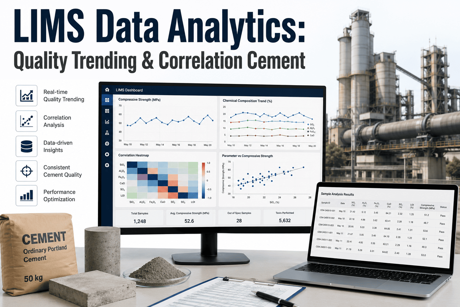
Correlation analysis is the analytical technique that converts LIMS data into diagnostic intelligence. When two variables move together across hundreds of observations, one is either causing the other or they share a common cause — and either finding is actionable. The matrix below shows the correlation relationships cement quality analytics most consistently surfaces from historical LIMS data, with the coefficient strengths reflecting what mature plants typically observe once the analytical layer is running against several months of clean data. These are the starting points for diagnostic investigation, not the finish line — but for most plants, even having them named and quantified is a step change from the tacit knowledge that only lives in the heads of the senior process engineers.
The last correlation on the matrix is the single most economically valuable finding LIMS analytics produces for cement operations. The 28-day strength is the property customers pay for, but it arrives 28 days after the material is made — long after the batch has been sold and delivered. The 1-day strength arrives while the material is still in the silo. When the correlation between 1-day and 28-day is strong for a specific plant and product grade, the 1-day result becomes a defensible predictor of the 28-day outcome. That prediction is what lets the plant hold or dispatch material on the day it is made rather than gambling that the 28-day number will land where expected.
Correlation strength is worth interpreting carefully. A strong positive correlation between, for example, kiln burning zone temperature and clinker C3S content does not by itself prove that raising the burning zone temperature will increase C3S — it establishes that the two move together across the plant's operating envelope. Cement quality analytics adds value by surfacing these relationships as measurable rather than assumed, but the physical mechanism behind each relationship still needs to be understood by the process engineering team before the correlation becomes an operational lever. The plants that get the most value from correlation analysis treat each new correlation the analytics surfaces as a starting point for engineering investigation, not a finished answer — which is what distinguishes analytics-informed decision making from analytics-substituted decision making.
The 4-Hour Rule: Why Trending Matters More Than Point Results
In cement production, there is typically a four to eight hour lag between when a process deviation occurs and when the lab result confirms it. During that window, the plant is either producing material that will need to be reworked, downgraded, or wasted — or it is producing acceptable material and nobody knows for sure. The 4-hour rule is the practical constraint that makes trending analytics dramatically more valuable than isolated point results: by the time a single out-of-spec result arrives, six or more hours of production have already happened at the drifting condition. The trend line arrives earlier because it is watching the direction of travel, not just the destination.
The trending advantage compounds across every quality parameter, every shift, every day. A plant running SPC-based trending catches drift a few hours earlier on average than a plant running only individual result checks, which sounds modest until multiplied by the number of quality events per year and the tonnage produced during the difference. Over a full year, the compounded difference typically shows up as measurable reduction in downgrade production, off-spec reworked material, and customer claims traced to marginal quality. The economic value of catching drift four hours earlier is not visible in any single event — it becomes visible in the annual variance report, where the plants running trending analytics consistently show tighter distribution around target values than plants relying on point-result flags alone.
Prediction: The 28-Day Strength Question Answered on Day One
Prediction is the highest-value analytics capability cement LIMS data enables, and 28-day strength prediction from 1-day results is the specific prediction with the clearest economic payback. The mechanics are straightforward: a regression model trained on several months of historical pairs of 1-day and 28-day strength results — segmented by product grade, and refined with additional inputs like Blaine fineness and clinker C3S content — produces a 28-day estimate at the point the 1-day result is available. Prediction accuracy typically exceeds 90 to 95 percent correlation with the actual 28-day result once the model is calibrated to the specific plant's historical data.
The operational impact of prediction is straightforward: material that would previously have been dispatched on faith and confirmed 28 days later can now be dispatched on a data-supported prediction of 28-day performance. Material that the prediction flags as at-risk of missing grade can be held for confirmation testing before shipping — avoiding the customer claim and reputational cost of a downgrade discovery weeks after delivery. Neither outcome is possible without the analytical layer on top of the LIMS data, but both are routine at plants that have deployed the prediction capability.
Prediction models also produce a second, less obvious benefit that shows up in raw material and process optimization. When the model can attribute predicted 28-day strength to specific input variables — clinker C3S content, Blaine fineness, sulfate level — the coefficients themselves become diagnostic. A shift in the coefficient linking C3S to 28-day strength across time can indicate that the underlying clinker mineralogy is changing in ways the routine testing was not catching. A stable coefficient combined with declining predicted strength points instead to a variable that the model is watching drift. Either interpretation is more actionable than the raw strength trend alone, and both fall out of the same analytical framework once it is running against several months of clean LIMS data. This is the payoff of treating LIMS analytics as a live capability rather than a one-time model build: the analytical framework keeps learning as new results arrive, and the diagnostic signal it produces keeps improving with the underlying data.