In modern manufacturing, cycle time variability is the silent profit killer that traditional engineering studies consistently fail to detect. While lean methodologies and time-and-motion studies have served the industry for decades, they lack the granularity to capture the complex interplay between operator skill, machine degradation, material inconsistencies, and environmental factors. Machine learning (ML) offers a transformative approach by analyzing thousands of data points per minute from sensors, PLCs, and MES systems, revealing patterns invisible to the human eye. This deep-dive guide explores how AI-driven cycle time analysis can reduce variability by 15-30%, directly improving OEE and throughput without capital expenditure. For enterprise decision-makers seeking a competitive edge, understanding these techniques is no longer optional. Book a Demo to see how iFactory applies ML to your production data.
Eliminate Hidden Cycle Time Waste
Machine learning identifies root causes of variability. Achieve consistent takt time and unlock hidden capacity.
The Hidden Complexity of Cycle Time Variability
Cycle time is rarely constant. Even in highly automated lines, minute fluctuations accumulate into significant throughput losses. Traditional time studies average observations, discarding the rich variance that holds diagnostic value. Machine learning models, particularly gradient boosting and random forests, can ingest high-frequency data from multiple sources: spindle load, temperature, operator scan rates, material batch properties, and even shift schedules. These models quantify the contribution of each variable to cycle time variance, often revealing surprising culprits such as a 2-second delay caused by a specific material supplier or a 1.5-second increase during the third shift. By decomposing variance, manufacturers can prioritize corrective actions with precision.
Moreover, ML models can predict cycle time for each work order before production begins, enabling dynamic scheduling and bottleneck prevention. This predictive capability allows planners to assign orders to the best-matched line configuration, reducing overall lead time. In one automotive parts plant, an iFactory implementation reduced cycle time standard deviation by 42% within eight weeks by identifying that a specific operator station was consistently slower due to ergonomic layout issues. The model flagged this station as a top contributor to variance, prompting a low-cost workstation redesign that yielded immediate gains.
Operator Influence
ML models detect subtle differences in operator technique, training gaps, and fatigue patterns. By correlating cycle time with operator ID, shift start time, and break schedules, factories can implement targeted coaching or rotation policies.
Machine Degradation
Spindle vibration, temperature rise, and power draw fluctuations precede cycle time increases. Predictive models flag these early signs, enabling proactive maintenance that stabilizes cycle time before quality is affected.
Material Variability
Incoming material properties—hardness, thickness, moisture content—directly impact processing time. ML models learn these relationships and can recommend batch sequencing to minimize cycle time swings.
Data Architecture for Cycle Time ML
Building a robust cycle time model requires a deliberate data architecture. The foundation is a time-series database capturing all relevant signals at a frequency of at least 1 Hz. Key data sources include: PLC cycle start/end timestamps, robot joint positions, conveyor speed, sensor readings (temperature, pressure, vibration), operator badge scans, material lot IDs, and quality inspection results. This data must be aligned in a single timeline, often requiring timestamp normalization across different systems. iFactory’s edge platform handles this harmonization automatically, creating a unified data lake ready for ML ingestion.
Feature engineering is the next critical step. Raw timestamps are transformed into meaningful features: cycle time per station, cumulative cycle time per product, time between cycles (idle time), and ratio of actual to ideal cycle time. Additional features capture external factors such as ambient temperature, humidity, and shift number. The target variable is typically the cycle time of the next unit or the deviation from a baseline. Models are trained on historical data and validated on a holdout set to ensure generalization. Regular retraining is essential as production conditions evolve.
| Data Source | Signal Type | Frequency | Use Case |
|---|---|---|---|
| PLC | Cycle timestamps | Per cycle | Baseline cycle time |
| Vibration sensor | RMS acceleration | 10 Hz | Machine health |
| Operator scanner | Badge ID | Per operation | Operator effect |
| Material lot system | Batch properties | Per lot | Material influence |
| MES | Work order data | Per order | Product mix impact |
Machine Learning Models for Cycle Time Analysis
Gradient Boosting (XGBoost, LightGBM)
These ensemble methods excel at capturing non-linear interactions between features. They handle missing data well and provide feature importance rankings, making them ideal for identifying root causes of cycle time variance. In practice, LightGBM can train on millions of rows in minutes, enabling near-real-time predictions.
Random Forest
A robust baseline model that reduces overfitting through bagging. Random forests offer excellent interpretability through feature importance plots and partial dependence curves. They are particularly useful when the dataset contains many categorical variables such as operator ID or shift.
Long Short-Term Memory (LSTM)
For sequences of operations, LSTM networks capture temporal dependencies. They can model how a delay in one station propagates downstream, predicting cycle time for the entire production line. LSTMs require more data and tuning but can achieve superior accuracy on complex lines.
Bayesian Models
When data is scarce or noisy, Bayesian approaches provide uncertainty quantification. They output a distribution of possible cycle times rather than a single point, enabling risk-aware decision-making. This is valuable for high-mix, low-volume environments.
Implementation Roadmap for Cycle Time ML
Data Audit & Connectivity
Assess available data sources, sampling rates, and quality. Install edge gateways to collect PLC and sensor data. Ensure timestamp synchronization across all systems.
Baseline & Feature Engineering
Calculate current cycle time distribution (mean, median, standard deviation). Engineer features from raw signals. Create a labeled dataset with cycle time as target.
Model Training & Validation
Train multiple candidate models. Use k-fold cross-validation to assess performance. Select the model with best RMSE and business interpretability.
Deployment & Real-Time Prediction
Deploy model to edge or cloud. Integrate predictions into MES or dashboard. Set up alerts for predicted cycle time deviations exceeding thresholds.
Continuous Improvement Loop
Monitor model drift and retrain monthly. Use SHAP values to explain predictions to operators and engineers. Iterate on feature set as new data becomes available.
Ready to Stabilize Your Cycle Time?
Deploy ML models that identify root causes in days, not months. Start your transformation now.
Case Study: Automotive Tier 1 Supplier Reduces Cycle Time by 22%
A mid-sized automotive supplier producing engine components faced chronic OEE losses due to cycle time variability. Their manual analysis could only attribute 40% of variance to known causes. iFactory deployed an ML solution that ingested data from 12 PLCs, 30 vibration sensors, and operator scan logs. Within three weeks, the model identified that 60% of cycle time variance was driven by three factors: material batch hardness (32%), operator experience level (18%), and a specific robot arm calibration drift (10%). The plant implemented a material pre-sorting system, a mentorship program for new operators, and a robot recalibration schedule. Result: cycle time standard deviation dropped from 4.2 seconds to 2.1 seconds, OEE rose from 72% to 81%, and scrap reduced by 15%. The ROI was achieved in four months.
Common Pitfalls in Cycle Time ML Projects
Ignoring Data Quality
Garbage in, garbage out. Without proper timestamp alignment and outlier handling, models will produce misleading results. Invest in data cleaning and validation pipelines.
Overfitting to Historical Patterns
Production environments change. A model trained on last year's data may fail after a new product launch or process change. Implement retraining workflows and monitor for drift.
Lack of Interpretability
Black-box models frustrate plant engineers. Use SHAP or LIME to explain predictions. Visualize feature contributions to build trust and drive action.
Neglecting Human Factors
Operators may resist changes suggested by ML. Involve them early in the process, explain the model's logic, and show how it makes their job easier. Change management is critical.
Frequently Asked Questions
How does ML differ from traditional cycle time analysis?
Traditional methods rely on stopwatch studies and average calculations, which miss subtle interactions between multiple variables. ML models analyze thousands of data points per second from diverse sources, detecting non-linear patterns and providing probabilistic predictions. For example, an ML model can identify that a 2-second delay occurs only when a specific operator works with a particular material batch on a machine that has been running for more than 4 hours. This level of granularity is impossible with manual studies. Learn more about our approach by booking a demo at Book a Demo.
What data infrastructure is needed to get started?
At a minimum, you need timestamped cycle start/end events from your PLCs or MES. Ideally, you also collect machine sensor data (vibration, temperature, power) and operator/material identifiers. iFactory's edge platform can connect to most industrial protocols (OPC-UA, Modbus, Siemens S7) and automatically normalizes timestamps. For support with data connectivity, visit iFactory Support. Our team can assess your current infrastructure and recommend a minimal viable data collection plan.
How long does it take to see results from a cycle time ML project?
Typical timelines range from 4 to 12 weeks depending on data availability and model complexity. The fastest wins come from simple linear models or gradient boosting on existing PLC data, which can be deployed in under a month. More complex deep learning models for highly variable lines may take 8-12 weeks. However, most clients see a 10-15% reduction in cycle time variance within the first two months. For a detailed timeline tailored to your factory, Book a Demo with our solution architects.
Can ML models handle high-mix, low-volume production?
Yes, but the approach differs. For high-mix environments, Bayesian models or hierarchical models that share information across similar product families work well. Feature engineering becomes critical—you need to encode product attributes (size, material, complexity) that influence cycle time. iFactory has deployed successful solutions in electronics and aerospace job shops with thousands of SKUs. The key is to have enough historical data for each product family. Contact us at iFactory Support to discuss your specific mix.
How do you ensure model accuracy over time?
We implement automated monitoring pipelines that track prediction error and feature distributions. When drift is detected (e.g., mean cycle time shifts by more than 5%), the model is retrained on recent data. Additionally, we recommend quarterly audits where domain experts review feature importance rankings to ensure the model still reflects physical reality. For ongoing support and model maintenance, visit iFactory Support.
Transform Your Factory Floor with AI-Driven Cycle Time Optimization
Join industry leaders who have reduced cycle time variance by over 30%. Let's discuss your specific challenges.