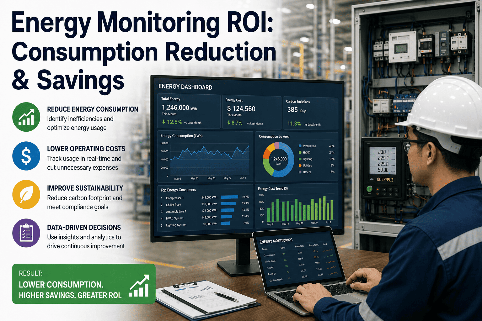
Most industrial facilities operate with a single utility meter at the property boundary, which means energy bills arrive as monthly summary totals that reveal nothing about where the energy was consumed, when it was consumed, or whether that consumption was necessary for production. This single-meter blindness is the primary reason that energy costs remain one of the largest controllable expenses in manufacturing that is rarely controlled with the same rigor applied to labor, raw materials, or maintenance. Energy monitoring systems that deploy sub-metering at the process and equipment level transform an opaque monthly bill into a continuous stream of actionable data that exposes waste, quantifies savings opportunities, and validates that efficiency initiatives are actually delivering the reductions they promise. The financial return from this visibility is not theoretical. Facilities that implement comprehensive energy monitoring consistently achieve 10 to 25 percent reduction in total energy consumption within the first 18 months, with the monitoring system itself paying for itself in 6 to 12 months from the savings it enables. Book a demo to see how iFactory makes energy consumption visible at every level of your operation.
Your Energy Bill Tells You What You Spent. Energy Monitoring Tells You What You Wasted.
iFactory deploys sub-metering intelligence across your facility to expose exactly where, when, and why energy is consumed, turning your utility cost from a monthly surprise into a daily management metric you can actively control.
Where Your Energy Dollars Actually Go in a Typical Manufacturing Facility
When a facility receives a single monthly energy bill, the only number visible is the total cost. What remains invisible is how that total breaks down across processes, equipment, and operational patterns. The following breakdown represents the typical energy consumption distribution observed across industrial facilities that have implemented comprehensive sub-metering, revealing that the largest cost categories are often the least understood because they have never been measured at the source. Understanding this distribution is the essential first step in prioritizing where monitoring investment will deliver the fastest and largest financial return.
The critical insight from this distribution is that the three largest categories, process heating, motor systems, and compressed air, together account for 72 percent of total energy cost but receive the least monitoring attention in most facilities because they are perceived as inseparable from the production process itself. Energy monitoring proves that significant portions of this consumption are not productive but rather waste hidden within processes that no one is measuring. iFactory makes these categories individually visible from day one of deployment, enabling targeted efficiency actions where the financial impact is largest.
Five-Step Framework to Calculate Your Energy Monitoring ROI Before You Invest
One of the barriers to energy monitoring investment is the perception that ROI is difficult to calculate before deployment because you do not yet know what you will find. In reality, ROI can be estimated with reasonable accuracy using the following five-step framework that relies on industry benchmark data for the savings potential within each energy category, adjusted for your specific facility characteristics. This framework has been validated against actual post-deployment results across more than 80 industrial facilities and consistently produces estimates within 15 percent of realized savings at the 12-month mark.
Four-Level Metering Hierarchy That Maximizes Visibility per Dollar Invested
Not all metering points deliver equal value. Deploying 500 meters without a hierarchical strategy produces massive data volumes with diminishing analytical returns because most of the meters are measuring loads too small or too aggregated to drive actionable decisions. The following four-level hierarchy defines the optimal metering architecture that maximizes the ratio of actionable insight to metering investment by ensuring that each level answers a specific management question and that lower levels are only deployed where the upper levels have identified an opportunity that requires finer granularity to address.
The most common deployment mistake is installing too many Level 4 meters before Level 2 and Level 3 data has identified where fine-grained measurement will deliver the highest return. A facility that deploys Level 1 and Level 2 first, analyzes the data for 60 to 90 days, and then selectively deploys Level 3 and Level 4 based on what the data reveals will achieve a higher ROI than a facility that deploys all four levels simultaneously based on engineering assumptions about where the waste is. iFactory supports this staged deployment approach by analyzing each level's data and recommending exactly where the next level of metering should be added to maximize financial return.
Peak Demand Profile: Where Your Money Is Made and Lost in 15-Minute Windows
For industrial electricity customers, the demand charge component of the monthly bill is often misunderstood or completely ignored, even though it typically represents 20 to 40 percent of total electricity cost. Demand charges are based on the highest 15-minute average power draw recorded during the billing period, meaning that a single 15-minute spike in consumption can set the demand charge for the entire month. Without real-time monitoring, facilities have no visibility into when these peaks occur or which equipment combinations create them. The following profile shows a typical industrial facility's demand pattern over a 24-hour period, with the peak demand window highlighted along with the controllable loads that could have been shifted to avoid it.
The fundamental insight from demand profile analysis is that peak demand is almost always a scheduling problem, not a technology problem. The equipment creating the peak is necessary for production, but the timing of when that equipment operates within a 2 to 3 hour window is flexible in ways that are invisible without real-time demand monitoring. Once the monitoring system reveals exactly when the peak occurs and which loads contribute to it, the corrective action is typically a procedural change in start-up sequencing, not a capital investment in new equipment. This makes peak demand management one of the highest-ROI applications of energy monitoring because the savings are immediate and the implementation cost is near zero once the visibility exists.
Energy-Per-Unit Benchmarking Across Production Lines and Shifts
Energy-per-unit is the single most powerful metric for driving accountability and continuous improvement in industrial energy management because it normalizes energy consumption against production output, eliminating the confounding effect of production volume changes. Without this normalization, a facility that reduces energy consumption simply because production declined will incorrectly believe it has improved efficiency. The following benchmark table shows the type of energy-per-unit analysis that becomes possible once sub-metering is deployed at the process area level, comparing performance across production lines, shifts, and time periods to identify where operational practices create efficiency differences that would otherwise remain hidden.
| Metric | Line A | Line B | Line C | Best Practice | Gap to Best |
|---|---|---|---|---|---|
| Electricity (kWh/unit) | 4.82 | 5.37 | 4.45 | 4.20 | Line B: +28% |
| Natural Gas (therms/unit) | 2.15 | 2.08 | 2.64 | 1.95 | Line C: +35% |
| Compressed Air (cfm-hours/unit) | 18.4 | 22.1 | 19.8 | 16.0 | Line B: +38% |
| Day Shift EPU Index | 100 | 100 | 100 | 100 | Baseline |
| Night Shift EPU Index | 108 | 119 | 112 | 100 | Line B Night: +19% |
| Weekend EPU Index | 124 | 131 | 128 | 100 | All lines elevated |
| Monthly Trend (6-month) | Stable | Worsening +4% | Improving -3% | Improving | Line B needs action |
This type of analysis, which is impossible without sub-metering at the process area level, reveals three critical findings that demand management attention. First, Line B is consistently the highest energy consumer per unit across all energy types, suggesting systemic operational differences that should be investigated by comparing its practices against Line C which is the best internal performer. Second, night shifts across all lines show 8 to 19 percent higher energy per unit compared to day shifts, indicating that either equipment is being operated differently at night or that support systems such as compressed air and cooling are running at full capacity despite lower production demand. Third, weekend operation shows the highest energy per unit across all lines, suggesting that batch processes started on Friday are running through the weekend with support systems at full load but production at reduced rates. Each of these findings represents a specific, actionable optimization opportunity that monitoring data has made visible.
Quantified Savings Potential by Energy Optimization Strategy
Energy monitoring does not save energy by itself. It enables savings by revealing the specific opportunities where energy is being consumed without productive value and by validating that corrective actions actually deliver the expected reduction. The following savings estimates represent the typical range of reduction achieved by each strategy when implemented using data from a comprehensive monitoring system. These are not theoretical maximums but observed results from facilities that have used monitoring data to identify, implement, and verify efficiency improvements. The percentage ranges reflect the variation between facilities with different starting efficiency levels and different levels of management commitment to acting on the data.
12-Week Deployment Timeline from Contract to First Savings
Energy monitoring systems do not require the extended implementation timelines associated with enterprise software deployments. Because the core value is derived from data collection and visualization rather than complex business logic or organizational process changes, a well-executed deployment can deliver actionable data within 12 weeks from contract signature. The following timeline shows the standard deployment sequence used by iFactory for manufacturing facility energy monitoring, with each phase building on the previous one and delivering incremental visibility that enables early savings even before the full system is operational.
The key principle of this timeline is that savings begin during Weeks 6 through 8 when Level 1 and Level 2 data first becomes available, not after the full deployment is complete. Peak demand management savings, which require only total facility visibility, can be implemented as soon as the Level 1 meter is validated. Area-level benchmarking and scheduling corrections can begin as soon as Level 2 data has established a 2 to 3 week baseline. The more targeted equipment-level savings enabled by Level 3 and Level 4 metering build on this foundation but are not a prerequisite for capturing the initial wave of savings that often pays for a significant portion of the monitoring system investment within the first quarter.
Common Questions About Energy Monitoring ROI
How accurate are the pre-deployment ROI estimates, and what happens if actual savings fall short of projections?
The five-step ROI framework described in this article consistently produces estimates within 15 percent of actual 12-month realized savings when applied using conservative assumptions from the lower end of industry savings ranges. However, the accuracy depends heavily on using your actual energy cost data rather than industry averages for the baseline, and on honestly assessing your facility's starting efficiency level. Facilities that have never monitored energy typically achieve savings at the higher end of the projected ranges because they start with more hidden waste. If actual savings fall short, it almost always indicates that the monitoring data identified opportunities but the organization did not act on them due to resource constraints or priority conflicts. The monitoring system did its job by revealing the opportunity, but the ROI realization requires management commitment to follow through on the identified actions. Book a demo to get a facility-specific ROI estimate.
What is the ongoing cost of maintaining an energy monitoring system, and does it require dedicated staff?
Ongoing costs for energy monitoring include software platform licensing, meter calibration and replacement on a 5 to 10 year cycle, communication infrastructure maintenance, and the labor cost of reviewing data and acting on findings. Annual ongoing costs typically range from 15 to 25 percent of the initial first-year investment. Dedicated energy management staff is not required for most mid-size facilities if the monitoring platform provides automated dashboards, alerts, and reports that integrate into existing operational roles. A typical model assigns energy data review responsibility to an existing engineer or supervisor who spends 2 to 4 hours per week reviewing automated reports, investigating alerts, and coordinating efficiency actions. The financial return from the monitoring system is typically 5 to 10 times larger than the ongoing cost, making the maintenance investment self-funding from the savings it protects. Contact support for ongoing cost modeling.
Can energy monitoring be deployed in stages, or does the full system need to be installed at once to deliver value?
Staged deployment is not only possible but is the recommended approach for most facilities because it allows data from each level to guide where the next level of metering investment should be focused. Starting with Level 1 utility entrance metering delivers immediate value through billing validation and real-time total demand visibility at a very low cost. Adding Level 2 process area metering 30 to 60 days later enables energy-per-unit tracking and cross-area benchmarking that identifies which areas warrant deeper investigation. Level 3 and Level 4 equipment and component metering are then deployed selectively based on what the upper levels reveal, ensuring that every additional meter is placed where the data will drive the largest financial return. This staged approach also spreads the capital investment over 6 to 12 months while delivering measurable savings from the earliest deployment stages. Book a demo to plan your staged deployment.
How does energy monitoring integrate with existing systems like SCADA, CMMS, or ERP?
Energy monitoring systems integrate with existing operational technology and enterprise systems at multiple levels to multiply the value of the data. Integration with SCADA systems allows energy data to be correlated with process conditions, enabling analysis of how process operating parameters affect energy consumption per unit of output. Integration with CMMS platforms allows energy monitoring alerts to automatically generate maintenance work orders when equipment degradation is detected through power consumption trending, closing the loop between energy anomaly detection and corrective action. Integration with ERP systems allows energy cost data to be allocated to production orders, cost centers, or product SKUs for accurate product costing. iFactory provides pre-built integration connectors for common SCADA, CMMS, and ERP platforms, enabling these data flows without custom development and ensuring that energy intelligence becomes part of your existing operational workflows rather than a separate standalone system. Contact support for integration architecture details.
What happens to the savings after the first year? Does the benefit diminish over time as the easy fixes are exhausted?
The first year typically captures the largest single-year savings because it includes the elimination of the most obvious waste such as compressed air leaks, failed steam traps, and peak demand scheduling corrections that are immediately visible once monitoring begins. However, savings do not diminish to zero after year one because the monitoring system provides two persistent value streams that continue indefinitely. First, it provides continuous validation that previously implemented savings are being maintained and not eroding as equipment drifts out of optimal settings or operational practices revert to pre-optimization habits. Facilities without monitoring typically lose 30 to 50 percent of achieved savings within 3 years because there is no mechanism to detect efficiency regression. Second, it enables ongoing fine-tuning as production mixes change, equipment is replaced, or new processes are added, each of which creates new optimization opportunities that only a continuously monitoring system can identify in real time. Book a demo to discuss long-term savings sustainability.
Every Kilowatt You Cannot See Is a Kilowatt You Cannot Control. Start Seeing All of Them.
iFactory deploys energy monitoring intelligence across your entire facility in weeks, not months, giving your operations team the real-time visibility and automated analytics needed to turn energy from a fixed cost into a managed variable that improves your bottom line every single day.