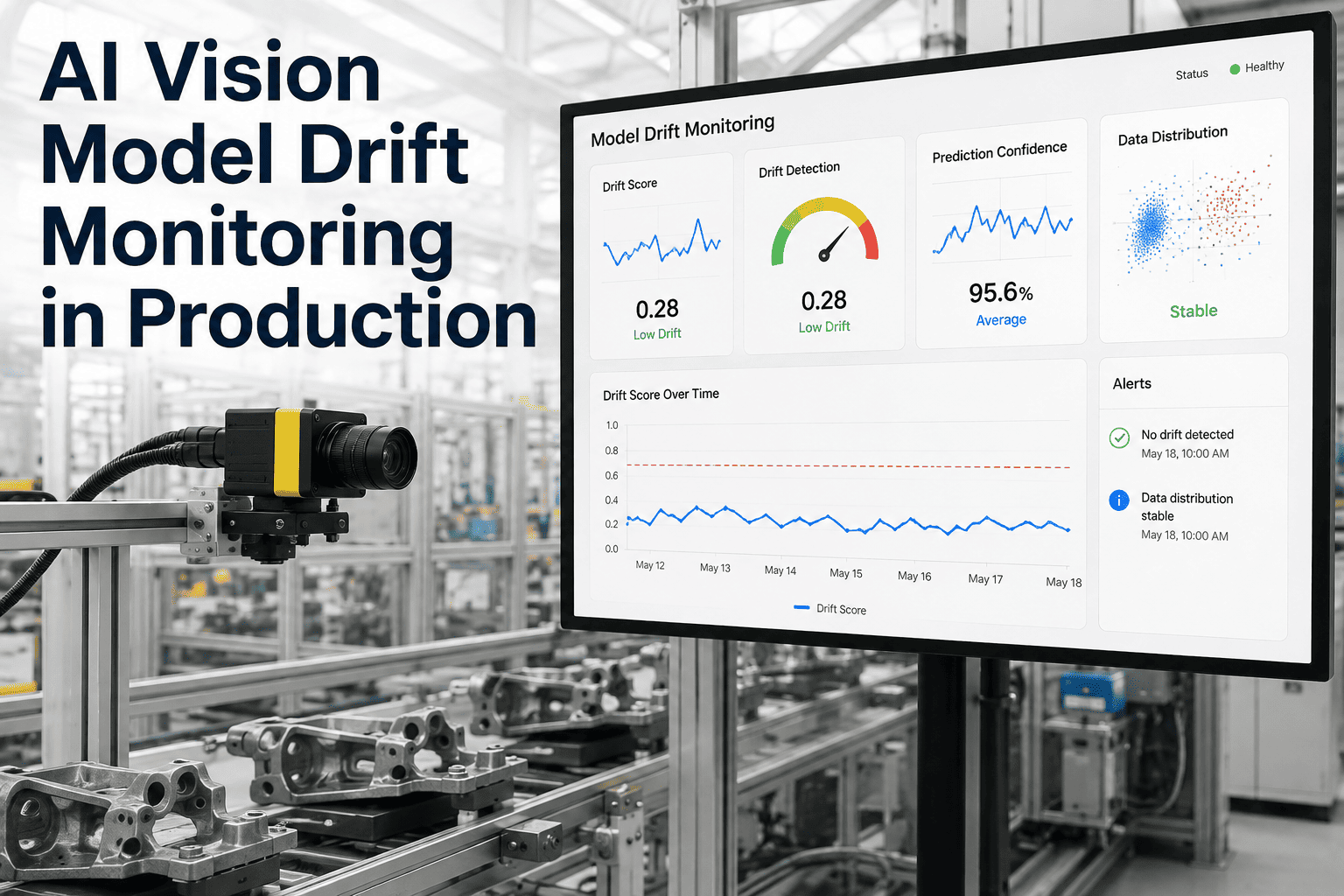
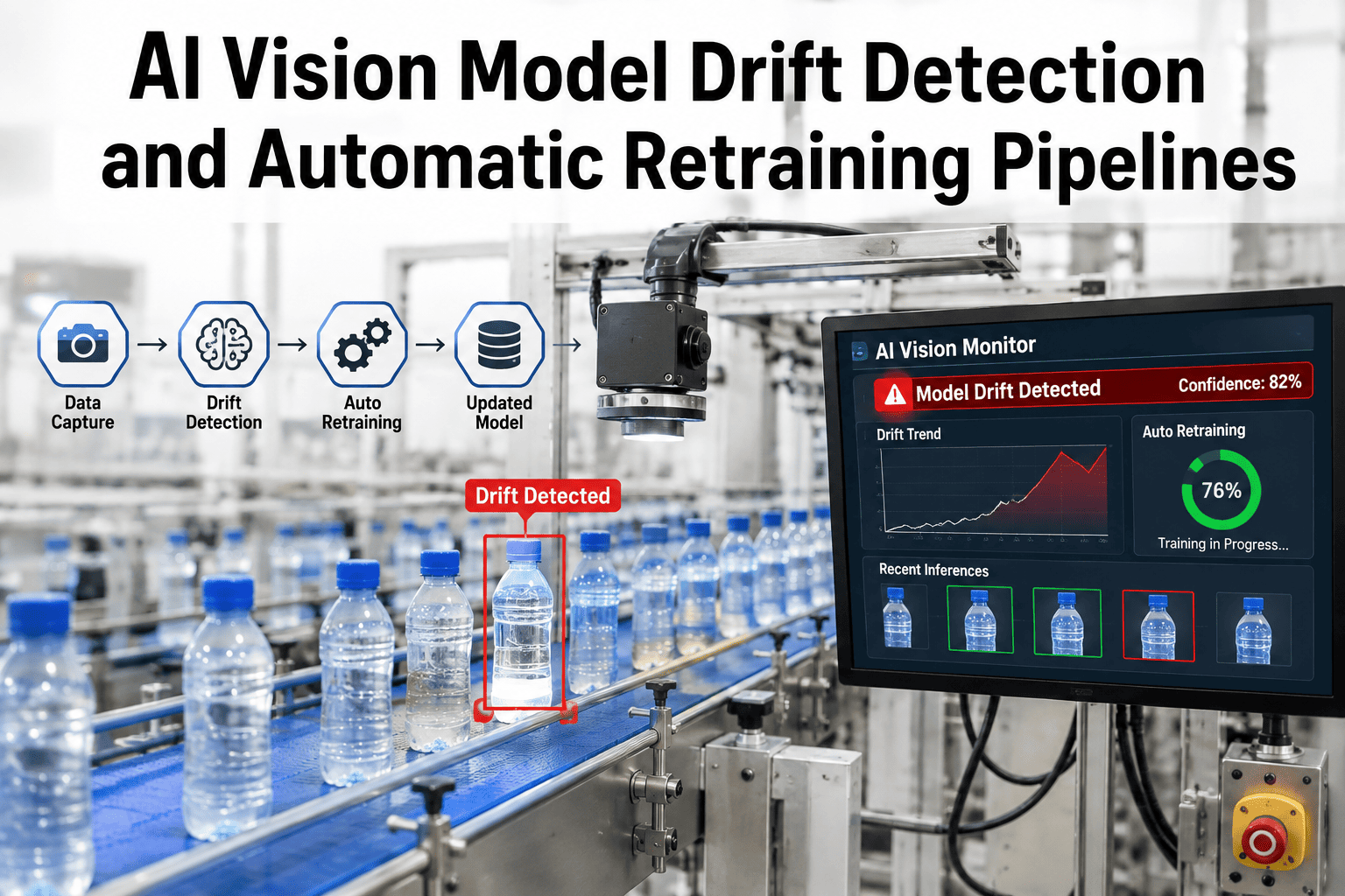
Every AI vision model that goes live in a factory starts its life at its best. Commissioning day accuracy is as good as it will ever be — the lighting matches training conditions, the parts match the training distribution, the camera is freshly calibrated. What almost nobody plans for is what happens next: month by month, the real world drifts away from the conditions the model was trained on, and detection accuracy quietly erodes without a single alarm going off. This is model drift, and in vision inspection it is far more dangerous than in most other AI applications because a drifting vision model does not fail loudly — it keeps returning confident predictions, just wrong ones, on a rising share of parts. Teams running AI inspection in production can book a demo to see how iFactory's drift monitoring layer catches this decay before it reaches the scrap line.
MODEL HEALTH · DRIFT DETECTION · PRODUCTION MONITORING
AI Vision Model Drift Monitoring in Production — Catch the Decay Before the Scrap Report Does
Vision inspection models degrade silently in production as lighting, materials, and process conditions shift away from training data — drift monitoring tracks confidence, detection rate, and distribution health continuously, so the model gets corrected before it costs you a shift's worth of missed defects.
LIVE MODEL HEALTH SIGNALS · MONITORED CONTINUOUSLY
Confidence Score
Tracked prediction by prediction
Detection Rate
Compared week over week
Distribution Shift
Flagged before it becomes an error
The Silent Killer: Why Drift Is the Hardest Failure to Notice
A vision model does not throw an exception when it drifts. It does not crash, log an obvious error, or stop the line. It keeps running, keeps returning predictions, and keeps assigning confidence scores — the failure mode is entirely statistical, buried inside a rising rate of missed defects or an unexplained creep in false rejects that looks, from the plant floor, exactly like noise. This is what makes drift categorically different from a hardware failure or a network outage: nothing visibly breaks, so nothing visibly demands attention, until the accumulated cost shows up somewhere else — a customer complaint, a scrap report anomaly, a quality audit finding.
Vision-specific drift research has documented this pattern directly, noting that quality inspection models can begin missing critical defects as the underlying distribution of input images shifts, and that monitoring performance alone is not sufficient to detect this kind of drift because performance metrics themselves lag the underlying shift. By the time the accuracy dashboard shows a problem, the causal shift in lighting, materials, or process has usually been active for weeks — the dashboard is reporting history, not warning of what's coming.
Anatomy of Drift: The Three Ways a Vision Model Loses the Plot
Not all drift is the same phenomenon wearing different clothes. Production ML research consistently distinguishes between three related but distinct failure modes, and knowing which one is active determines what kind of fix actually works. Confusing the three is the most common reason a "quick retrain" fails to fix a drifting inspection station — the team retrained against the wrong signal.
TYPE 1
Data Drift (Covariate Shift)
The statistical distribution of the images themselves changes — new lighting, a new camera, a supplier's material with a different surface texture — while the actual relationship between "what a defect looks like" and "is it a defect" stays the same. Data drift means input distributions shift over time while the input-output relationship stays constant, which is why this type is often correctable with recalibration rather than a full relabel-and-retrain cycle.
Typical fix: Recalibrate imaging conditions or fine-tune on recent production images
TYPE 2
Concept Drift
The relationship between the visual pattern and the correct answer actually changes — a defect definition gets tightened by a new customer spec, a new failure mode emerges that looks visually similar to something previously classed as acceptable, or a process change makes a previously-defective pattern now within tolerance. This is the deeper failure mode because no amount of recalibration fixes it — the labels themselves have moved.
Typical fix: Relabel affected examples and retrain the decision boundary
TYPE 3
Environmental & Sensor Drift
The physical capture conditions degrade gradually — a lens accumulates dust, an LED array ages and dims, a camera sensor's white balance calibration wanders. None of this is a change in the world being inspected, only in how faithfully the sensor is capturing it, but the model sees it as though the world itself had shifted.
Typical fix: Sensor maintenance, recalibration, and hardware health checks
The Signal Stack: What a Properly Monitored Vision Model Actually Tracks
Effective drift monitoring is not one metric — it is a layered stack of signals, each catching a different stage of decay. Waiting for the top-level accuracy number to move is the slowest possible warning system, because by the time aggregate accuracy visibly drops, the underlying shift has usually been compounding for weeks. A production-grade monitoring stack watches earlier, faster-moving signals that give lead time before the top-line number ever budges.
01
Confidence Score Distribution
A healthy model returns confidence scores clustered tightly near its decision extremes — very confident on clear passes, very confident on clear fails. As drift sets in, the distribution spreads, and more borderline scores start appearing in the middle. Watching the shape of the confidence distribution, not just its average, surfaces drift before it shows up as a wrong decision.
02
Detection Rate Stability
Tracking the rate at which the model actually flags known defect types over time — if a station is finding a consistent percentage of a known defect category in week one and a meaningfully lower percentage by week twelve, that gap is a real cost even if nobody noticed a single specific miss along the way.
03
False Reject Rate Trend
A progressive rise in false rejects with no obvious upstream cause is one of the earliest ground-level drift symptoms. A station historically rejecting a stable low single-digit percentage of parts that silently climbs over several weeks is very often reporting drift, not a genuine change in part quality.
04
Feature-Level Distribution Shift
Comparing the statistical distribution of internal model features extracted from live production images against the distribution recorded at training time. Feature drift is often best detected on these internal embeddings rather than raw pixels, because a shift in the extracted-feature distribution catches lighting, sensor, and domain changes that pixel-level statistics miss entirely.
05
Statistical Divergence Metrics
Formal statistical tests quantify how far current production data has moved from the training baseline. The Population Stability Index and Kullback-Leibler divergence are the industry-standard metrics here, with a rising PSI trend acting as an early quantified warning long before the shift becomes visible in day-to-day operations.
CONTINUOUS MONITORING · EARLY WARNING · NO SURPRISE RETRAINS
Stop Discovering Drift From a Quality Escape
iFactory's drift monitoring layer tracks confidence distribution, detection rate, and statistical divergence continuously on every deployed inspection model — flagging decay weeks before it shows up as a scrap spike or a customer claim, so corrections happen on your schedule instead of an angry customer's.
The Drift Timeline: How a Healthy Model Quietly Becomes an Unreliable One
Drift is rarely a single dramatic event — it is a slow accumulation that crosses a threshold nobody was watching for. The timeline below traces the typical arc of an unmonitored vision model from commissioning through the point where the cost becomes visible on a scrap report, showing exactly where each of the earlier warning signals would have surfaced the problem if anyone had been tracking them.
WEEK 0
Commissioning — Peak Accuracy
Model validated against a curated dataset under ideal, matched conditions. Accuracy is at its lifetime best and the confidence distribution is tight and well-separated. This is the number everyone remembers and nobody expects to change.
WEEK 2–6
Silent Divergence Begins
Real production introduces small, cumulative differences from the training distribution — a slightly different supplier lot, seasonal ambient light changes, early sensor grime. Top-line accuracy has not visibly moved. Confidence score distribution has already started spreading, invisible without dedicated monitoring.
WEEK 6–10
Early Ground-Level Symptoms
False reject rate begins a slow, easy-to-dismiss climb. Detection rate on rarer defect types starts to soften. Operators notice "a few more rejects than usual" but attribute it to a bad batch of raw material rather than the model itself.
WEEK 10–14
Statistical Divergence Crosses the Threshold
Formal drift metrics like PSI have now crossed the accepted significance threshold, if anyone is computing them. Detection rate on the most common defect category has measurably softened compared to week one — a gap with real, compounding cost even though nobody has flagged a specific miss yet.
WEEK 14+
The Cost Surfaces
A scrap report anomaly, a customer complaint, or a quality audit finally makes the drift visible at the business level. Root-cause investigation now has to work backward through three months of accumulated shift to figure out what actually changed and when — an investigation that continuous monitoring would have made unnecessary by flagging the shift in week three.
Detection Approach vs Response Time: Why Waiting for the Accuracy Dashboard Costs the Most
Different monitoring approaches catch drift at very different points in its lifecycle, and the gap between them is measured in real production cost. The table below compares the common approaches to catching model decay in production vision systems, from the least to the most proactive.
| Monitoring Approach |
What It Catches |
Typical Lead Time |
Where It Falls Short |
| No monitoring — react to complaints |
Only failures severe enough to trigger a customer or audit escalation |
None — reactive only |
Cost has already compounded for weeks before anyone knows |
| Periodic manual review — scheduled accuracy checks |
Aggregate accuracy drops visible at review intervals |
Days to weeks, depending on review cadence |
Labor intensive, tedious to sustain, easy to skip under production pressure |
| Top-line accuracy dashboard — automated but shallow |
Aggregate performance drops once they are large enough to move the average |
Weeks — the average is a lagging signal |
Reports history rather than warning of what is compounding underneath it |
| Confidence & distribution monitoring — continuous, signal-layered |
Early distribution spread, feature drift, statistical divergence before accuracy visibly moves |
Days — flags shift as it begins accumulating |
Requires an instrumented monitoring layer built into the deployment |
The pattern across every production ML maintenance framework is the same — the earlier the monitoring layer sits in this chain, the more lead time the quality and engineering teams get to correct the drift before it becomes a scrap event. Continuous signal-layered monitoring is not a luxury feature bolted onto a vision system after the fact — it is the difference between a planned recalibration and an unplanned customer escalation.
A Realistic Scenario: The Rejection Rate That Crept for Ten Weeks
A tier-one automotive component plant runs an AI vision station inspecting weld quality on a high-volume assembly line. The model launches with strong validated accuracy and runs cleanly through the first month, and the quality team moves on to other priorities, checking the dashboard only during the monthly review cycle. Over the following ten weeks, nothing dramatic happens — no equipment failure, no obvious process change, no single bad shift that anyone would flag in a handover note.
What actually happens is quieter. A new coil supplier introduces a subtly different surface reflectivity that the model was never trained against. Week over week, the confidence score distribution on borderline welds spreads a little wider, and the false reject rate creeps from a stable two percent toward three, then four percent — each individual week's change small enough to blend into normal shift-to-shift noise. By week ten, operators are manually re-verifying a meaningfully larger share of rejected parts than they were in week one, quietly absorbing the cost in labor hours nobody has line-itemed as a model problem. The monthly dashboard review finally flags an accuracy number that has moved enough to notice, and the ensuing investigation takes another two weeks to trace the false reject climb back to the supplier changeover.
With continuous confidence-distribution and statistical divergence monitoring active from day one, the same shift would have triggered an alert around week two or three — the confidence distribution spreading is a leading indicator that shows up long before the aggregate false reject rate has moved enough to notice on a monthly review. The fix in both cases ends up being the same, a targeted recalibration against recent production images from the new supplier's coil stock. The difference is entirely about when the fix happens — as a five-minute scheduled recalibration in week three, or as a two-week root-cause investigation in week twelve after ten weeks of elevated false rejects have already cost real labor hours and manual re-verification.
Building a Drift-Resilient Inspection Program: Four Practices That Actually Work
Monitoring alone is not enough — drift detection only delivers value when it initiates a response. The plants that keep AI vision accuracy stable over years, not just at commissioning, share a small set of operating practices that turn detection signals into corrective action before cost accumulates.
01
Establish a Reference Baseline That Actually Gets Reused
Every monitoring signal is a comparison against something — a reference distribution captured at validated, healthy performance. That baseline needs to be preserved and versioned, not just used once at commissioning, so every future drift check has a real point of comparison rather than a vague sense of "seemed fine before."
02
Set Thresholds Tied to Business Cost, Not Statistical Convention
A generic statistical threshold treats every drift signal the same regardless of what it actually costs the plant. Thresholds tuned against the real cost of a false reject versus a missed defect on that specific line make the alerting system genuinely actionable instead of a wall of noise that gets ignored.
03
Route Alerts to a Defined Response, Not Just a Dashboard
A drift alert that lands in an inbox nobody checks delivers zero value. Effective programs route each alert type to a specific action — recalibration for environmental drift, targeted relabeling for concept drift, sensor maintenance for hardware degradation — with clear ownership for who acts on it.
04
Close the Loop With Scheduled, Not Emergency, Retraining
Plants with mature drift programs treat model refresh as a scheduled maintenance activity, informed by ongoing signal trends rather than triggered only by a visible failure. This shifts the entire cost structure from expensive emergency response back to routine, budgeted upkeep.
Frequently Asked Questions
How is drift monitoring different from just watching the accuracy dashboard?
Top-line accuracy is a lagging signal — it only moves once enough individual predictions have gone wrong to shift the average, which typically means the underlying shift has already been active for weeks. Drift monitoring watches earlier, faster-moving signals like confidence score distribution, feature-level statistical divergence, and detection rate stability on specific defect categories, all of which tend to shift well before the aggregate accuracy number visibly changes. Teams that want to see this layered monitoring against their own inspection data can
book a demo to walk through it directly.
Does every drift signal mean the model needs to be retrained?
No — not every distribution change actually affects model accuracy, and teams should confirm real impact before committing to a retraining cycle. Some drift signals point to environmental or sensor issues correctable with a simple recalibration or hardware check, while others reflect a genuine concept shift that does require relabeling and retraining. A properly instrumented monitoring layer distinguishes between these cases instead of treating every statistical wobble as a retraining trigger.
How much lead time does continuous monitoring actually buy compared to periodic manual review?
The gap is significant and compounds with review cadence — a monthly manual review can leave a drift condition unnoticed for weeks while cost accumulates in the background as elevated false rejects, unnecessary manual re-verification labor, or missed defects reaching downstream processes. Continuous signal-layered monitoring flags the same shift within days of it beginning, turning what would have been a multi-week root-cause investigation into a scheduled, low-cost recalibration.
Can drift monitoring work on a vision model we did not originally build with iFactory?
Yes — drift monitoring is fundamentally about comparing live production data and model outputs against a reference baseline, which is an approach that layers onto an existing deployed model without requiring it to be rebuilt from scratch. Teams running vision inspection on any platform can contact
iFactory support to discuss integrating continuous drift monitoring on top of their current inspection stations.
What is the difference between data drift and concept drift, and why does it matter for the fix?
Data drift is a change in what the images look like — new lighting, new materials, new sensor characteristics — while the actual rule for what counts as a defect stays the same, and it is often correctable with recalibration or lightweight fine-tuning. Concept drift is a change in the rule itself — a defect definition shifts, a new failure mode emerges, or a process change moves the pass-fail line — and it requires relabeling and a genuine retrain because no amount of recalibration can fix a decision boundary that has moved. Diagnosing which type is active is the first step in choosing the right, cost-appropriate fix.
MODEL HEALTH · CONTINUOUS MONITORING · PLANNED NOT EMERGENCY FIXES
Give Your Inspection Model the Same Uptime Discipline You Give Your Machines
iFactory monitors confidence distribution, detection rate stability, and statistical divergence on every deployed vision model continuously — surfacing drift while it is still a five-minute recalibration, not a two-week root-cause investigation after a customer escalation.