Steel Plant Energy Monitoring & Demand Control | iFactoryAI
By David Cook on August 4, 2026
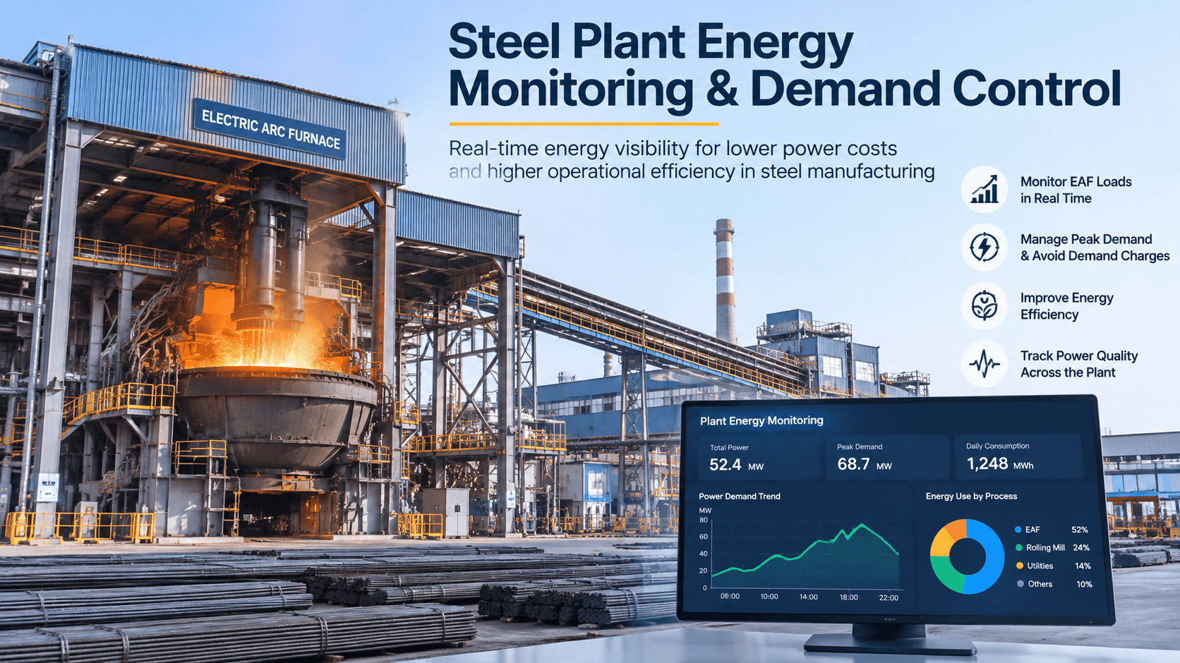
A single 150-ton electric arc furnace pulls 60,000 kWh in roughly an hour — enough electricity to power an average U.S. household for six years, drawn down in one heat cycle. At peak arc-on, the same furnace can hit 100 MW of instantaneous demand, equal to a small city. That is the reality of steel mill electricity: it is not just a big monthly bill, it is a live grid event, and every megawatt of peak demand shows up twice — once on the energy line and once on the demand-charge line. The plants that run best-in-class hit 300 kWh per ton. The plants that don't run around 400. On 500,000 annual tons, that 100 kWh gap is $2.8 million a year in wasted electricity before you count the coincident peak charges triggered by two furnaces going bore-in at the same time. Most melt shops still run fixed power recipes regardless of scrap mix, tap on operator experience, and review energy performance after the shift. That gap between what the meter is doing right now and what the shift report shows is where the recoverable margin lives — and it lives per heat, per shift, per crew. iFactory Peak Demand Manager is built to close it: sub-cycle sampling on every furnace, real-time coincident-peak tracking across the whole plant, and per-heat kWh/ton attribution before the next charge lands.
iFactory Peak Demand Manager for Steel
Cut kWh/Ton and Kill Coincident Peaks — Heat by Heat
Real-time EAF power monitoring, per-heat energy attribution, and coincident peak control across furnaces, rolling mills, and auxiliaries — before the demand charge locks in for the month.
An electric arc furnace does not consume power evenly. One heat cycle is a sharp four-phase profile: bore-in, main melt, refining, and tap. Each phase has its own load, its own duration, and its own recoverable minutes. This is what a typical 60-minute heat looks like on the meter.
One EAF heat — 60 min, ~60,000 kWh, up to 100 MW peak
Foamy slag holding heat — small gains, real minutes
Tap
30-40 MW
Cool-down — starts the clock for the next heat
Where Steel Energy Money Actually Leaks
Steel-plant electricity spend is not one big leak. It is five different leaks that stack together. Naming them individually is how you attack each one on its own terms.
01
Coincident peak demand
Locked for the month
Two furnaces going bore-in at the same time creates a peak that sets the demand charge for 30 days. Nobody scheduled it — it just happened.
02
kWh/ton drift
100 kWh/t possible
Same steel grade, same scrap mix, same crew — but heat A ran 380 kWh/t and heat B ran 445. Nobody knows why until end-of-shift, and by then eight more heats have run.
03
Off-peak arbitrage missed
10-30% tariff spread
Time-of-use tariffs vary by hours of factor 2-3×. EAFs can flex — but only if the schedule reflects the tariff, and most schedules don't.
04
Auxiliary background load
15-25% of total
Rolling mills, fume systems, cooling water pumps, compressed air — draws 15-25% of the plant total, rarely benchmarked, and running full even when furnaces are down.
05
Power quality penalties
Poor PF surcharge
EAFs create harmonics and reactive power distortion. Poor power factor triggers utility surcharges and damages downstream equipment — invisible on the shift report.
Want to see which of the five is costing you the most? Book a demo — bring one week of meter data and we'll break it down.
The Peak Demand Trap
Utility demand charges are not just a slice of the bill — they can be 30-50% of the total electricity spend on a steel mill. And they are set by the single 15-minute or 30-minute peak in the billing period. One coincident event costs you 30 days.
WITHOUT DEMAND MANAGEMENT
Furnaces scheduled by production, not by grid
Two EAFs go bore-in simultaneously — 180 MW peak
15-min average peak sets demand charge for the month
Nobody sees the peak until the utility bill arrives
Same month, same crews, same waste — repeat
WITH PEAK DEMAND MANAGER
Live coincident load visible across all furnaces
Warning at 65 MW per unit, hard alert at 80 MW threshold
Furnace 2 bore-in delayed 4 min — total peak stays at 95 MW
Auxiliaries shed automatically during high-load windows
Monthly demand charge protected before the peak fires
Per-Heat Attribution — Why Two Identical Heats Cost Differently
Two heats of the same steel grade, same scrap mix, same crew can end up 50 kWh/t apart. The difference lives in tap-timing decisions, foamy slag quality, power-off gaps between charges, and burner-oxygen coordination. Attributing every heat to its actual drivers is how kWh/ton drift stops being a mystery.
Heat variable
Scrap mix density
±30 kWh/t
Light scrap needs more bore-in time; DRI blends change the power profile. Recorded against actual charge composition, not assumed.
Heat variable
Power-off time
+13 kWh/t per 5 min
Gaps between charges cool the furnace and cost kWh on the next arc-on. Continuous logging catches every delay.
Heat variable
Foamy slag stability
±25 kWh/t
Foamy slag acts as an insulating blanket — good foam saves energy, weak foam radiates it. Trended by arc voltage and stability index.
Heat variable
Tap temperature
+7 kWh/t per 10°C
Every degree over target is wasted energy. Attributed per heat, per grade, per crew — patterns show which crews consistently over-tap.
Heat variable
Oxygen/carbon injection
-20 to -40 kWh/t
Chemical energy from oxygen and carbon coordinated with electrical arc — imbalance wastes both. Live coordination benchmark.
Heat variable
Electrode consumption
Track kg/t
Electrode wear tied to arc regulation and slag conditions. Tracked heat-by-heat so wear anomalies become work orders, not surprises.
How Peak Demand Manager Runs the Loop
Cutting steel energy costs is not a report exercise. It is a live loop: measure at sub-cycle rates, decide during the heat, act before the peak locks in.
01
Sub-Cycle Sampling
Furnace MW, kVAr, harmonics, and PF captured at sub-cycle rates from existing meters and transformers.
02
Coincident Peak Tracking
Live plant-total load rolled up across furnaces, rolling mills, and auxiliaries — the number that sets the demand charge.
03
Warning + Threshold Alert
Warning band at 65 MW per unit, hard alert at 80 MW plant total — before the 15-min average locks a peak in.
04
Coordinated Action
Furnace bore-in staggered, auxiliaries shed automatically, dispatchers see the total in one view — the peak doesn't happen.
05
Per-Heat Attribution
Every heat closes with kWh/t attributed to scrap, power-off, tap temperature, and crew — logged for benchmarking and coaching.
What Peak Demand Management Delivers
Energy is 15-20% of steel production cost. Every point recovered is protected margin — and unlike scrap price, it is entirely in your control. These are the outcomes plants typically see after moving from monthly bills to live peak and per-heat management.
$2.8M
Energy gap closable
on a 500K t/yr EAF at 100 kWh/t recovery
30-50%
Bill share is demand
every peak avoided is protected margin
Live
Per-heat attribution
kWh/t decomposed to actual drivers
Grid
Ready
ISO/RTO peak signals integrated
Curious what a 50 kWh/t recovery and one avoided coincident peak is worth on your plant? Talk to our steel energy team — we'll size it against your tariff.
Frequently Asked Questions
How much energy can we actually recover on our EAF?
The gap between typical (400 kWh/t) and best-in-class (300 kWh/t) is 100 kWh/t. On a 500,000-ton annual plant, that gap alone is worth about $2.8 million a year in electricity — before counting demand-charge avoidance. Realistic first-year gains are usually 30-60 kWh/t through per-heat attribution, tap-temperature control, power-off management, and better oxygen/carbon coordination. The rest comes over 12-24 months as coaching and process discipline compound.
What exactly is a coincident peak and why does it matter?
Utility demand charges are set by your highest 15-minute or 30-minute average load in the billing period. When two furnaces go bore-in at the same time, you can spike the plant total to 180 MW even though each furnace is running normally. That single 15-minute window sets the demand charge for the whole month — and often for the whole billing year, depending on the tariff. Peak Demand Manager watches the plant-total live and coordinates furnace timing so coincident spikes never happen.
Do we need to change our furnaces or add new instrumentation?
No. Peak Demand Manager reads from your existing meters, PTs and CTs, and transformer monitors. Sub-cycle sampling on the electrical side, plus DCS or Level 2 for furnace phase data. On most modern EAFs the tags are already there — connection is a matter of days, not months.
How does this handle time-of-use and real-time tariffs?
The engine ingests your utility tariff structure — energy rate by hour, demand charge, coincident peak windows, power factor penalties, and any RTO peak signals. Every heat is costed in real time against the current tariff, and scheduling recommendations account for both the demand risk and the current energy price. Off-peak arbitrage becomes explicit, not accidental.
Can we see it running on our own plant before committing?
Yes. Bring one furnace and one month of meter and heat data. We'll build the per-heat baseline, compute the coincident-peak history, and show which peaks would have been avoided and how many kWh/t your best crews are already recovering vs. the fleet average. Book a demo and we'll walk it live on your data.
Stop discovering peaks on the utility bill.
See Coincident Peak & Per-Heat Energy On Your Own Furnace
Bring one furnace and one month of meter and heat history. We'll compute the coincident-peak profile, per-heat kWh/ton attribution, and the tariff-cost breakdown — with the specific peaks that would have been avoided and the crews already recovering the gap.