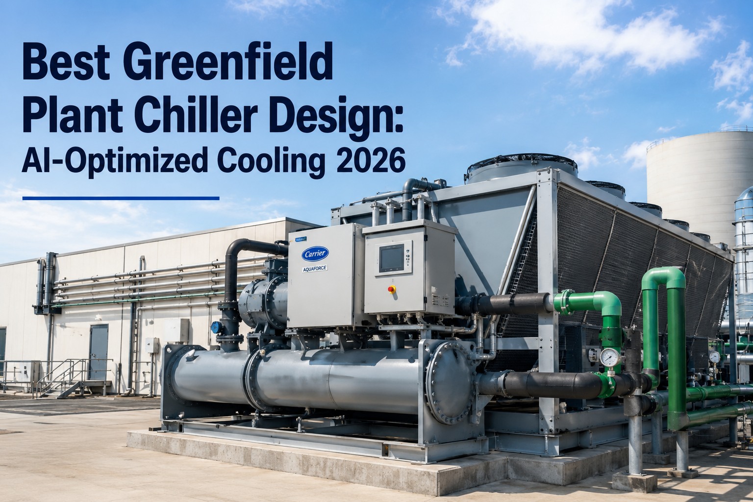
A greenfield plant's chiller system is the largest single controllable energy load in most industrial facilities — accounting for 30–50% of total facility electricity in process-intensive operations. The difference between a poorly specified chiller plant running at 1.0 kW/ton and an AI-optimized system running at 0.5–0.6 kW/ton is not marginal: on a 300-ton plant at $0.12/kWh running three shifts, that gap costs $190,000 per year in excess electricity. Getting the design right at FEED — chiller type, redundancy model, free cooling integration, AI control architecture, and refrigerant selection — determines whether that gap ever closes.
Design your greenfield chiller plant with iFactory — AI-optimized cooling architecture, redundancy modeling, and free cooling integration scoped before your MEP engineer finalizes the chilled water one-line.
2026 Chiller Plant Performance Benchmark
The kW/Ton Gap: Where Your Chiller Plant Will Land — and Why It Matters
kW/ton is the single most important chiller efficiency metric. The gap between an unoptimized and AI-optimized plant compounds every hour of operation for the life of the facility.
- Fixed-speed compressor
- No load forecasting
- No free cooling integration
- Variable speed drive
- Rule-based controls only
- Partial load optimization
- Magnetic bearing compressor
- Demand-based staging
- Cooling tower optimization
- Predictive load sequencing
- Free cooling economizer active
- Dynamic setpoint optimization
Calculations based on 300-ton plant, 6,000 hr/yr operation, $0.12/kWh. AI-optimized vs. unoptimized = $139K annual savings — payback on AI controls typically under 18 months.
Chiller Type Selection: The Design Decision That Locks in 20-Year Efficiency
Chiller type is the most consequential greenfield design decision — it determines the efficiency ceiling, refrigerant trajectory, compressor reliability profile, and minimum part-load performance. Three compressor technologies dominate industrial greenfield selection in 2026, each with a distinct efficiency, cost, and maintenance profile.
Scroll Compressor
- Simple, reliable — few moving parts
- Limited part-load efficiency (no VSD range)
- Best for small process cooling loads
- High maintenance cost per ton at scale
Screw Compressor
- VSD-capable — good part-load efficiency
- Widely available, serviceable globally
- Slide valve capacity control standard
- Oil management required — additional PM scope
Centrifugal / Magnetic Bearing
- Oil-free magnetic bearings — near-zero PM
- Outstanding part-load efficiency (IPLV)
- Native AI control integration — sensor-dense
- Highest lifecycle ROI at 200+ ton scale
of total facility electricity consumed by chiller plant in process-intensive manufacturing
improvement in annual energy consumption achievable through intelligent multi-chiller staging and AI sequencing (Johnson Controls, 2026)
best-in-class efficiency target for AI-optimized centrifugal chiller plants with free cooling integration in 2026
coefficient of performance achievable with modern magnetic bearing centrifugal chillers vs. COP 3–4 in older fixed-speed systems
Need chiller type matched to your process load profile and budget? Book a chiller design session with iFactory — we calculate cooling load, select compressor type, and model 5-year TCO before your MEP engineer specifies equipment.
Redundancy Architecture: Designing for Zero Unplanned Cooling Loss
Chiller redundancy is not about adding spare capacity — it is about designing a system that remains fully operational when any single component fails, without sacrificing part-load efficiency during the 95% of hours when all chillers are running. The two most common greenfield configurations have opposite failure modes.
Single Large Chiller + Spare
- On failure: 15–30 min cooling loss while standby starts
- Operates at poor part-load efficiency (100% unit at 40% load)
- Single point of failure in compressor, controls, and piping
- Cold standby may not start — reliability untested until needed
Multiple Smaller Chillers — Lead-Lag-Standby
- On failure: standby activates in 90–120 seconds automatically
- Multiple smaller chillers operate at higher part-load efficiency
- AI staging sequences chillers optimally at every load point
- Warm standby reliability tested routinely via lead-lag rotation
Greenfield rule: Three units at 50% capacity each (N+1 = N×50% + 1 spare) is the preferred configuration for most AI factory chiller plants — it delivers N+1 redundancy, excellent part-load efficiency, and three-way AI staging optimization. Size each unit for 50–60% of peak load, not 100%.
Need redundancy modeling for your chiller plant? Talk to iFactory's cooling design team — we run the redundancy simulation and size each chiller for the configuration that optimizes both reliability and part-load efficiency from day one.
Free Cooling Integration: The Design Detail That Pays Back in Year 1
A water-side economizer integrated into the chiller plant allows the cooling tower to reject heat directly to the chilled water loop — bypassing the compressor entirely during cooler ambient conditions. For a manufacturing plant running 6,000+ hours annually, compressor-free cooling hours in cooler months represent 15–30% of total cooling energy, returned at near-zero marginal cost. Designing the economizer bypass into the plant at FEED costs a fraction of retrofitting it after commissioning.
at 54–60°F
at 44–50°F
AI-Optimized Chiller Design — Engineered for 0.5 kW/Ton from Day 1
iFactory designs your greenfield chiller plant for AI-optimized performance from commissioning — chiller type selection, redundancy modeling, free cooling integration, AI control architecture, and predictive PM sensor suite, all specified before your MEP contractor prices the chilled water system.
AI Chiller Optimization: What the Control System Manages Continuously
AI chiller optimization is not a single control action — it is a continuous coordination of six interdependent variables, each of which affects overall plant kW/ton. Static rule-based controllers handle one or two variables at fixed setpoints. AI systems optimize all six simultaneously, in real time, against a predictive model of the next 4–24 hours of load.
Chilled Water Supply Temperature Setpoint Reset
AI raises chilled water supply temperature during cooler ambient conditions or lower load periods — reducing compressor lift and improving COP by 3–8% for every 2°F of setpoint increase, without compromising process temperature requirements.
Condenser Water Temperature Optimization
AI lowers condenser water temperature by increasing cooling tower fan speed and flow — reducing chiller lift. The optimal condenser setpoint is not fixed; it varies with wet bulb temperature, chiller loading, and tower fan energy cost. AI finds the economic optimum every 5 minutes.
Chiller Sequencing and Load Distribution
In multi-chiller plants, AI determines how many chillers run and at what load — keeping each unit in its efficiency sweet spot (typically 60–80% of full load) rather than running one at 100% and one at 20%. Dynamic staging reduces total plant kW by 10–20% versus fixed lead-lag rules.
Pump Speed Optimization (Variable Primary Flow)
AI controls chilled water and condenser water pump speeds based on differential pressure and actual flow requirements — eliminating the fixed-speed energy waste that consumes 10–15% of chiller plant electricity in unoptimized systems. Every 10% pump speed reduction cuts pump energy by ~27% (affinity law).
Predictive Load Forecasting
AI models next-hour and next-shift cooling demand from production schedules, weather forecasts, and historical patterns — pre-staging chillers 15–30 minutes before load arrives rather than reacting after supply temperature rises. Eliminates temperature excursions during shift changes and production startups.
Free Cooling Economizer Dispatch
AI monitors ambient wet bulb temperature against a real-time free cooling threshold model — activating the water-side economizer bypass when ambient conditions allow compressor-off operation, and modulating partial economizer contribution when ambient is in the hybrid range. Maximizes compressor-free hours annually.
Want AI optimization configured for your chiller plant from commissioning day one? Book an AI cooling controls session with iFactory — we specify the sensor architecture, control logic, and CMMS integration before your chiller vendor finalizes the controls package.
Expert Perspective
The gap between a poorly performing chiller plant running at 0.8–1.0 kW/ton and an optimized plant running at 0.5–0.6 kW/ton is not marginal — it is the difference between facilities that control their largest utility cost and facilities that don't. The greenfield window is the only opportunity to design AI optimization, free cooling integration, and predictive monitoring into the chiller plant at engineering cost rather than retrofit cost. Plants that miss this window spend years doing energy audits to recover savings that could have been designed in on day one.
average energy savings from optimized chiller plants — GSA/PNNL benchmark across large industrial facilities
reduction in total carbon footprint achievable with AI-optimized chiller plant continuous monitoring
typical payback on AI chiller optimization controls — versus 5–7 year payback on chiller hardware replacement
0.5 kW/Ton from Day 1 — Design It In, Not Retrofit It Later
iFactory's chiller design service covers type selection, redundancy modeling, free cooling integration, AI control architecture, and predictive PM sensor suite — delivered as a complete chiller plant specification before your MEP contractor prices the chilled water system. The energy savings you design in at FEED cost nothing to implement. The savings you retrofit cost 3–5× more and arrive years late.
Frequently Asked Questions
What is kW/ton and what is a good target for a greenfield AI factory chiller plant?
kW/ton measures how many kilowatts of electricity the chiller consumes per ton of cooling output — the primary efficiency metric for chiller plants. Lower is better. Unoptimized air-cooled plants run at 1.0–1.2 kW/ton; standard water-cooled plants achieve 0.65–0.85 kW/ton; AI-optimized centrifugal plants with free cooling integration achieve 0.5–0.6 kW/ton. For a 300-ton plant running 6,000 hours annually at $0.12/kWh, the difference between 1.1 and 0.55 kW/ton is $139,000 per year — recovered before the first major service interval.
What chiller type should a greenfield AI factory specify?
Magnetic bearing centrifugal chillers are the optimal choice for AI-native manufacturing plants with loads above 150 tons and 24/7 operation profiles. They achieve 0.48–0.65 kW/ton (COP 5.4–7.3), require near-zero oil maintenance, integrate natively with AI control platforms through dense sensor suites, and deliver the highest lifecycle ROI despite higher upfront cost. For loads below 60 tons, scroll compressors remain cost-effective. Mid-range loads of 60–500 tons are best served by VSD screw compressors as a cost-performance balance.
How does free cooling integration save energy in a manufacturing chiller plant?
A water-side economizer allows the cooling tower to reject heat directly to the chilled water loop when ambient wet bulb temperature falls below 40°F — bypassing the compressor entirely. In temperate climates, this delivers 1,200–2,500 compressor-free hours annually, representing 15–30% of total cooling energy at near-zero marginal cost. AI integration with weather forecast data pre-positions the bypass valve before ambient conditions change, eliminating the temperature excursions that occur with manual or threshold-based switching. Designing the economizer into the plant at FEED costs a fraction of retrofitting it post-commissioning.
What redundancy configuration is recommended for a greenfield plant chiller system?
Three chillers at 50% capacity each (N+1 with each unit at half-load) is the preferred configuration — delivering N+1 redundancy, excellent part-load efficiency since each unit operates near its COP peak, and three-way AI staging optimization. On failure, the warm standby activates in 90–120 seconds versus 15–30 minutes for a cold standby. Each unit also receives regular operation through lead-lag rotation, confirming standby reliability before it is needed in an emergency.
What sensors does an AI chiller optimization system require?
The minimum sensor suite for AI chiller optimization includes: chilled water supply and return temperature at the plant and at each major load; condenser water supply and return temperature; chilled water flow meter (ultrasonic or electromagnetic); compressor power meter per chiller; cooling tower fan power and approach temperature; ambient wet bulb temperature sensor; and differential pressure across the chilled water distribution system. These twelve measurement points give the AI model the inputs to compute real-time kW/ton, optimize setpoints, sequence chillers, and detect efficiency drift — typically flagging fouled condensers or tube scaling 3–6 weeks before efficiency penalty becomes significant in the monthly energy bill.