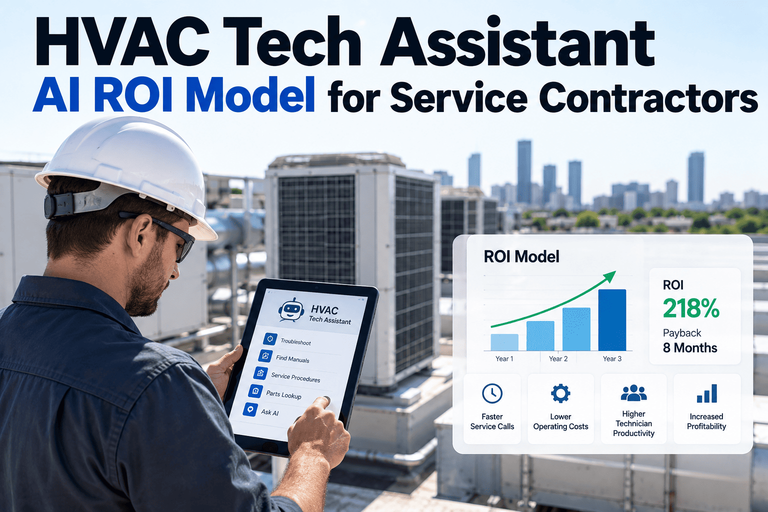
Every service contractor evaluating a technician assistant eventually asks the same blunt question: does this pay for itself, and how fast. The honest answer depends on three levers that move independently — first-time fix rate, callback volume, and technician productivity — and the contractors who get a clear answer are the ones who model all three together rather than eyeballing one metric in isolation. A properly built ROI model for HVAC tech assistant AI turns those three levers into a single payback number contractors can defend to ownership. Contractors who want a model built around their own numbers can start with a conversation with iFactory support.
Three Levers, One Payback Number: What This Actually Returns
First-time fix rate gain, callback reduction, and technician productivity, quantified together into a worked payback model under ten months.
Why a Single Metric Never Tells the Full ROI Story
It is tempting to model ROI around one number — usually first-time fix rate, because it is the easiest to track. But a service contractor that only improves first-time fix while callback rate and technician productivity stay flat is leaving most of the value on the table. The three levers interact: a higher first-time fix rate reduces callbacks almost automatically, and a technician who diagnoses faster completes more tickets per day, which compounds the labor savings beyond either metric alone.
A complete model tracks all three, weights them by what they actually cost the business, and rolls them into a single payback figure that can be defended to ownership or a finance team without hand-waving.
Where the Savings Actually Come From
Each lever contributes savings in a different way, and the relative size of each contribution shapes how the payback timeline unfolds. The breakdown below reflects a typical modeled deployment for a mid-size commercial service contractor running twenty-five to forty trucks.
Build the Model Around Your Own Fleet
Book a 30-minute walkthrough and we will run a payback model using your truck count, ticket average, and current callback rate.
A Worked Payback Timeline
Below is how a payback timeline typically unfolds for a mid-size commercial contractor, tracking cumulative savings against the deployment cost month by month.
Rollout begins
First-time fix gain visible
Callback rate drops measurably
Productivity gains compound
Cumulative savings cross cost
The Model Inputs That Actually Move the Number
A defensible ROI model is built from real operational inputs, not industry averages pulled from a generic slide. The table below shows the inputs that matter most and how each one shifts the payback timeline.
| Input | Typical Range | Effect on Payback |
|---|---|---|
| Fleet size | 15–60 trucks | Larger fleets spread deployment cost across more tickets, shortening payback |
| Current first-time fix rate | 55%–75% | Lower starting rates leave more room for gain, improving the payback case |
| Average ticket value | Varies by market and segment | Higher-value tickets amplify the dollar impact of every avoided callback |
| Current callback rate | 8%–18% | Every point of reduction removes a full truck roll's cost from the ledger |
| Average tickets per tech per day | 3–6 | Even modest per-ticket time savings compound across a full day and a full fleet |
A Composite Scenario: The Model Ownership Actually Signed Off On
A regional commercial service contractor running 32 trucks evaluated a technician assistant with a starting first-time fix rate of 64% and a callback rate of 13%. The contractor's finance lead was skeptical of a generic vendor ROI slide and asked for a model built from the fleet's actual ticket volume and average job value before approving any spend.
The resulting model projected a first-time fix rate gain to roughly 78% within the first two quarters, a callback rate reduction to under 7%, and a modest productivity gain of about 0.4 additional tickets per technician per day once diagnostic time shortened. Rolled together against the fleet's actual numbers, the model showed cumulative savings crossing the deployment cost at month nine — inside the ten-month range typical for a fleet this size, and specific enough that finance signed off without further negotiation.
Common Mistakes That Make an ROI Model Unconvincing
Using Industry Averages Instead of Fleet-Specific Numbers
A model built on generic benchmarks is easy for a finance team to dismiss. The convincing version uses this fleet's actual ticket volume, average job value, and current callback rate.
Modeling Only First-Time Fix Rate
Ignoring callback reduction and productivity gains understates the real return and makes the payback window look longer than it actually is.
Assuming Full Gains From Day One
Adoption ramps over the first several months as technicians build trust in the tool. A model that assumes instant full-strength gains overstates early savings and undermines credibility.
Leaving Out Deployment and Change-Management Cost
A payback figure that ignores rollout time, training, and integration effort is not a real payback figure. Those costs belong in the model from the start, not as a footnote.
Do You Have What You Need to Build a Real Model
You know your current first-time fix rate and callback rate
These two numbers are the foundation of the model. If they are not currently tracked, a rough estimate from recent CMMS data is enough to start.
You know your average ticket value and tickets per technician per day
These figures translate rate improvements into actual dollars, and most CMMS or billing systems can produce them directly.
Finance or ownership has a payback window they consider acceptable
Knowing the target payback window up front — six months, twelve months, eighteen — shapes how the model should be framed and which levers to emphasize.
Sensitivity Analysis: What Happens When Assumptions Change
Every ROI model rests on assumptions, and a model worth trusting shows how the payback number moves when those assumptions shift, rather than presenting a single fixed figure as though it were guaranteed. The most useful version of a contractor's model runs a handful of scenarios side by side — a conservative case where adoption ramps slowly and gains land at the low end of the typical range, a base case built from the fleet's actual current numbers, and an upside case where technician adoption is fast and gains compound more quickly than average.
Fleet size interacts with the model in a way that is worth understanding before committing to a number. A larger fleet spreads the fixed cost of deployment and training across more trucks and more tickets, which tends to shorten the payback window even when the per-technician gains are identical to a smaller fleet's. This is one reason a contractor running sixty trucks and a contractor running fifteen trucks can see meaningfully different payback timelines from the exact same underlying improvement in first-time fix rate.
The starting point matters just as much as the fleet size. A contractor already running a strong ninety percent first-time fix rate has much less room to improve than one running sixty percent, and the model should reflect that honestly rather than projecting the same percentage-point gain regardless of where a fleet is starting from. The most credible models cap projected improvement based on realistic industry ceilings, rather than extrapolating a flat improvement rate that would imply an unrealistic near-perfect outcome.
Seasonal variation is another factor worth building into the model rather than ignoring. HVAC service volume swings meaningfully between peak cooling season and shoulder months, and a payback model that only accounts for average monthly ticket volume can understate the speed of early gains during a high-volume season or overstate them during a slow one. Building the model around the actual seasonal pattern a contractor's business follows produces a timeline that holds up under real scrutiny rather than one that looks good only in the aggregate.
How This ROI Model Complements, Not Replaces, Operational KPIs
A payback model is a planning and approval tool, built to answer the specific question of whether and when a deployment pays for itself. It is not meant to replace the operational KPIs a contractor already tracks week to week, and treating the two as separate but connected is what keeps both useful over the life of a deployment. The ROI model sets an expectation before rollout; the ongoing operational dashboard is what confirms whether reality is tracking to that expectation once the tool is actually live.
First-time fix rate, callback rate, and average tickets per technician per day are usually already tracked in some form by any contractor running a CMMS, which makes them a natural bridge between the pre-rollout model and post-rollout reality. Reviewing these same three metrics on a monthly cadence after go-live, and comparing the actual trend line against what the model projected, gives a contractor an early warning if adoption is lagging or if the gains are tracking ahead of plan and the model was conservative.
It is worth building in a deliberate checkpoint, typically around the three and six month marks, where the actual numbers are compared directly against the model's projected curve rather than just the final payback date. A model that projected a first-time fix rate gain reaching seventy-eight percent by month six but is actually sitting at seventy-two percent by that point is not necessarily a failure — it may simply mean payback lands a month or two later than projected — but catching that gap early gives a contractor the chance to investigate whether it is an adoption issue, a training gap, or simply a slower ramp than the base case assumed.
Contractors who treat the ROI model as a living document, revisited and adjusted as real data comes in rather than filed away after the initial approval, tend to get more long-term value from it. The same model structure used to justify the initial deployment can be reused to build the business case for expanding into a new region, a new asset class, or a larger share of the fleet once the pilot data validates the original assumptions.
Common Objections From Finance and How the Model Answers Them
A finance lead reviewing a technology spend request has heard optimistic vendor projections before, and the most common objection raised against any new field technology ROI model is a version of "these numbers assume everything goes perfectly." The strongest response to that objection is not a more confident assertion of the numbers but a model that has already shown its work — the conservative, base, and upside scenarios described earlier, built from the fleet's own current metrics rather than a vendor benchmark, with the assumptions stated plainly enough that finance can challenge any one of them directly.
A second common objection concerns opportunity cost — whether the same investment might return more if spent on additional trucks, additional technician headcount, or a different operational improvement entirely. This is a fair comparison to make explicitly rather than avoid, and a well-built model can be extended to show the marginal cost of adding a truck and technician versus the marginal cost of improving the productivity of the existing fleet, letting finance weigh both options on the same basis rather than evaluating the technology spend in isolation.
A third objection often centers on switching or exit costs — what happens financially if the deployment underperforms the model and the contractor needs to unwind it. Addressing this directly, including what data and process changes would need to be reversed and what the realistic sunk cost would be in a worst-case scenario, tends to reassure a skeptical finance reviewer more effectively than simply asserting confidence in the projected outcome.
Presenting the model alongside a short list of the specific operational changes that will actually be tracked post-rollout — not just projected but the exact metrics that will be pulled from existing systems — turns the ROI conversation from a one-time approval pitch into an ongoing accountability structure that finance teams tend to respond to more favorably than a static projection presented once and never revisited.
Comparing This Model Against Other Technology Investments
A finance team rarely evaluates a single technology proposal in a vacuum, and a contractor building an ROI model for a technician assistant should be prepared for it to be weighed against other competing uses of the same budget, whether that is a fleet vehicle upgrade, a new CMMS platform, or additional marketing spend aimed at growing ticket volume. Framing the technician assistant model in the same payback and risk terms used to evaluate those other investments makes for a far more persuasive comparison than presenting it in isolation with its own unique set of metrics.
One useful framing is comparing the cost per technician per month against the cost of achieving an equivalent productivity gain through headcount alone. Hiring and training an additional technician carries its own ramp time, recruiting cost, and ongoing payroll burden, and a model that shows the technology investment achieving a comparable productivity lift at a lower and more predictable cost per technician tends to resonate with a finance team already familiar with the true cost of adding headcount in a tight labor market.
Risk profile is another dimension worth addressing directly in the comparison. A headcount investment carries its own risk in the form of turnover and the multi-month ramp time before a new hire reaches full productivity, while a technology investment's risk is more concentrated in the adoption curve during the first ninety days. Presenting both risk profiles honestly, rather than only detailing the risk of the option being pitched, tends to build more credibility with a skeptical reviewer than a one-sided pitch.
Contractors who have successfully secured budget for this kind of investment often note that the deciding factor was not the size of the projected return but the specificity and defensibility of the model itself — a number built from the fleet's own data, with assumptions stated plainly and a clear plan for tracking actual results against the projection, tends to win approval even when a competing proposal shows a larger headline return built on less rigorous assumptions.
Frequently Asked Questions
What is a realistic payback window for a technician assistant deployment?
For a mid-size commercial service fleet in the range of twenty-five to forty trucks, a properly modeled deployment typically shows cumulative savings crossing the deployment cost inside ten months, driven by the combined effect of first-time fix rate gain, callback reduction, and technician productivity. Smaller fleets or fleets with a lower average ticket value may see a longer window, while larger fleets with higher call volume often see payback sooner. A model built from your own fleet's numbers is the only way to get a figure worth planning around, and iFactory can build that model by connecting with support to review your data.
Which lever typically contributes the most to ROI — fix rate, callbacks, or productivity?
First-time fix rate gain is usually the largest single contributor because it prevents costs before they occur, followed by callback reduction, with technician productivity gains compounding on top of both. The exact split shifts based on a fleet's starting callback rate — a contractor starting from a high callback rate will often see that lever contribute a larger share of total savings than the typical breakdown.
How long does it take to see the first measurable improvement after rollout?
First-time fix rate improvements are usually the earliest measurable signal, often visible within the first two to three months as technicians build familiarity with the tool and adoption ramps. Callback rate reduction tends to lag slightly behind, since it depends on a full cycle of jobs completed and any recurring issues resurfacing or not. Productivity gains are typically the last to fully compound, becoming clearest in the second and third quarters.
Does the ROI model account for training and change-management time?
Yes, a properly built model includes rollout time, technician training, and integration effort as real costs against the payback timeline rather than treating deployment as instantaneous and free. Leaving these costs out produces a payback number that looks better on paper but does not hold up once a finance team or ownership reviews it closely.
Can a smaller contractor with fewer than fifteen trucks still get a positive ROI?
Smaller fleets can still see a positive return, though the payback window is typically longer since deployment cost is spread across fewer tickets. The model math still works the same way — first-time fix rate, callback reduction, and productivity gains still apply per technician regardless of fleet size — it simply takes more months for cumulative savings to cross the smaller fleet's total deployment cost. Book a demo to see a model sized specifically to a smaller fleet.
Get a Payback Model Built From Your Actual Fleet Numbers
iFactory will build an ROI model using your truck count, ticket value, and current callback and first-time fix rates — not a generic industry benchmark. Book a walkthrough to see your number.