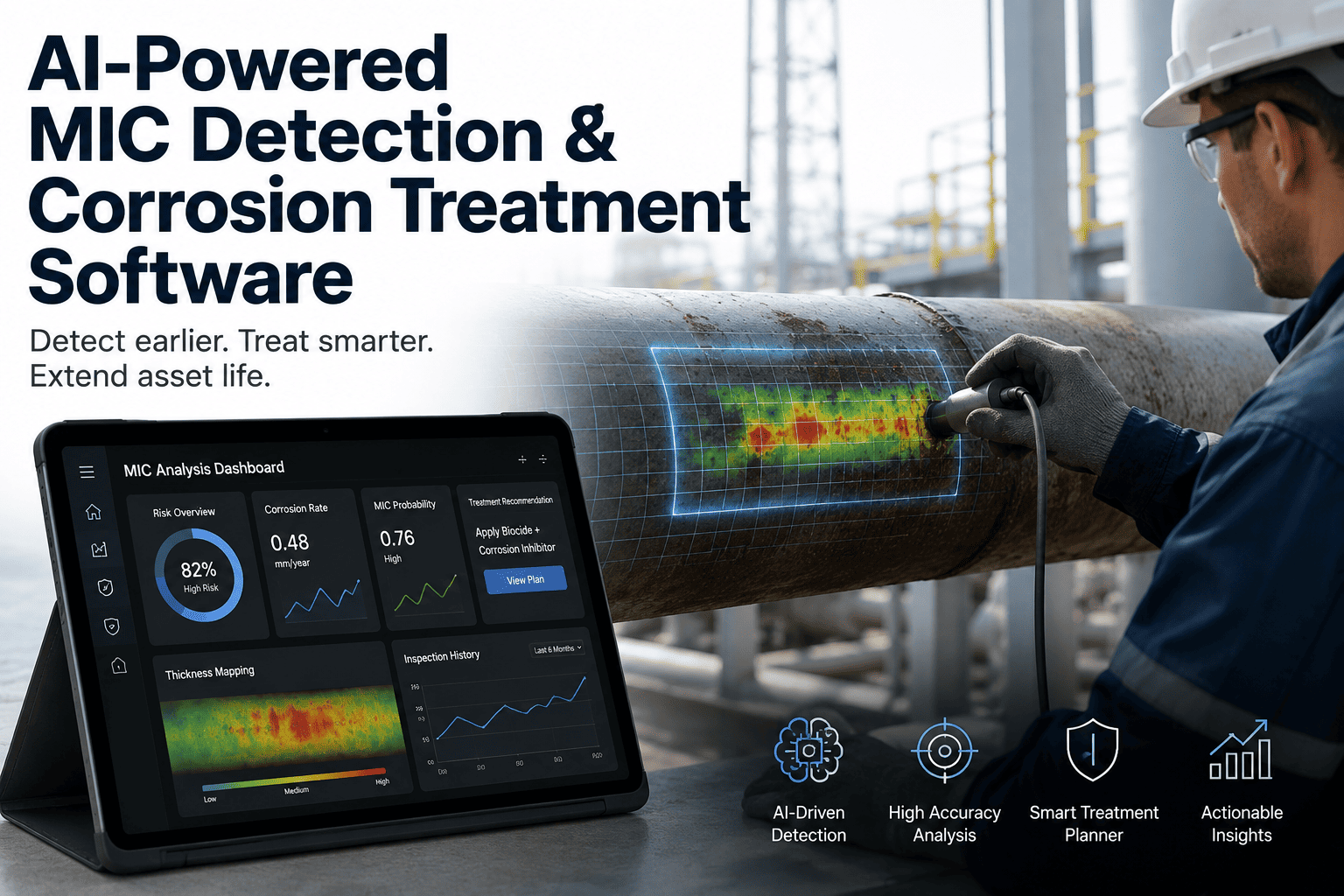
A pipeline can pass every scheduled ultrasonic thickness check and still be losing wall thickness at ten times the expected rate underneath a patch of biofilm nobody scraped off. Microbiologically influenced corrosion does not follow the smooth, predictable curves that general corrosion models assume — it pits fast, hides under deposits, and shows up in isolated spots that a handful of CML readings can miss entirely. Most operators still treat MIC as three separate problems: a water chemistry report from the lab, a biocide dosing log from operations, and a corrosion coupon pulled once a quarter. None of those three data sets talk to each other, which is exactly why MIC keeps finding the gaps. See how correlated MIC monitoring works on your system before the next isolated pit becomes a leak.
Three Data Sets. One Corrosion Mechanism. Zero Correlation — Until Now.
Water chemistry, biofilm activity, and corrosion rate each tell part of the MIC story. AI correlation software fuses all three into a single risk score per segment, catching the mechanism weeks before a coupon or a CML survey would.
Why MIC Outpaces General Corrosion Models
Standard corrosion allowance calculations assume a roughly uniform wall loss rate. MIC breaks that assumption in almost every case, which is why pipe that looks fine on paper can fail without warning.
higher localized pitting rate under an active MIC colony compared to the surrounding general corrosion rate
of unexplained internal corrosion failures in water-handling systems trace back to a microbial mechanism on later investigation
typical lag between the first detectable rise in sulfate-reducing bacteria activity and a measurable pit forming
The Three Data Streams a MIC Model Actually Needs
No single measurement confirms MIC on its own. A rising bacteria count without a corrosion signal is often background noise; a corrosion signal without a biofilm read could just as easily be erosion or CO2 attack. Correlating all three closes that gap.
Water Chemistry
Sulfate, dissolved oxygen, pH, chloride, and nutrient load set the conditions a microbial colony needs to establish and grow. Trending these values flags where the environment is turning favorable for MIC before any bacteria count confirms it.
Biofilm & Bacteria Activity
ATP bioluminescence testing, molecular qPCR counts for sulfate-reducing and acid-producing bacteria, and biofilm probe data measure how active the colony actually is, not just whether bacteria are present in a sample.
Corrosion & Metal Loss Data
Coupon weight loss, ER probe readings, and UT/CML thickness surveys confirm whether biological activity is translating into actual wall loss, and at what rate, on the segment being watched.
MIC Isn't One Mechanism — It's a Family of Them
Different bacteria types produce different corrosion signatures, and the right treatment strategy depends on knowing which one is actually driving the metal loss on a given segment.
Find Out Which Segments Are Trending Toward MIC
iFactory reviews your water chemistry history, biofilm sampling data, and last twelve months of corrosion readings to show exactly which segments carry active microbial risk right now.
Isolated Testing vs. Correlated AI Monitoring
Running water chemistry, biofilm testing, and corrosion coupons as three separate programs means three separate reports land on three separate desks, often weeks apart.
Optimizing Biocide Treatment Instead of Guessing at It
Biocide programs fail for predictable reasons — wrong dose, wrong timing, wrong chemistry, or a resistant colony that adapted around a stagnant rotation. AI correlation gives treatment decisions an actual feedback loop.
Dose Optimization
Kill-rate trending after each treatment shows whether the current dose is actually achieving target biocide contact time and concentration at the point of application.
Resistance Detection
A declining kill-rate trend across successive treatments with the same chemistry flags a colony that may be adapting, prompting a rotation before the program stops working entirely.
Timing Correlation
Cross-referencing water chemistry shifts with biofilm regrowth rate identifies the actual regrowth window for a given system, rather than relying on a generic calendar interval.
Cost Reduction
Segments with consistently low microbial activity can move to a reduced treatment frequency, freeing budget for the segments actually showing elevated risk.
What a Correlated Alert Actually Looks Like
A produced water line running through a low-flow gathering segment showed a slow sulfate rise over five weeks — nothing dramatic, and nothing that would have triggered a standalone chemistry alarm on its own. At the same time, ATP readings from the nearest biofilm sample point began climbing, and the ER probe two hundred feet downstream started showing a corrosion rate nearly triple the segment average. Individually, each signal sat within a plausible normal range. Correlated together against the segment's own baseline, the model flagged an active SRB colony developing at week three, four weeks before a scheduled coupon pull would have caught it and roughly six weeks before the pit would likely have reached actionable depth. The response was a targeted biocide slug and a follow-up UT scan, both completed inside a planned maintenance window instead of an emergency dig.
Rolling Out MIC Correlation Across a System
Most operators start with the segments carrying the highest consequence of failure and the least amount of existing instrumentation, then expand coverage as the model proves out.
Phase 1 — Baseline and data audit
Existing water chemistry, coupon, and probe history is pulled together and reviewed for gaps, since a model needs enough historical data on each segment to establish what normal actually looks like.
Phase 2 — Priority segment instrumentation
Segments with known low-flow zones, dead legs, or a prior MIC-related failure get continuous ER probes and more frequent biofilm sampling first.
Phase 3 — Correlation model tuning
Alert thresholds are tuned against your treatment response times and lab turnaround, so a flagged segment reaches the maintenance team with enough lead time to schedule biocide or inspection work.
Phase 4 — Systemwide expansion
Coverage extends to secondary segments using route-based sampling combined with the continuous instrumentation already proven on the priority segments.
Where MIC Programs Usually Go Wrong
Treating Bacteria Counts as the Whole Story
A high bacteria count without a corrosion signal often just means the colony hasn't reached an aggressive phase yet, not that treatment can wait.
Fixed Biocide Calendars
A generic 30 or 60 day dosing schedule ignores the fact that regrowth rate varies significantly by segment temperature, nutrient load, and flow.
Sampling Only Accessible Points
Dead legs and low-flow branches are the most MIC-prone locations and are frequently the same locations that get skipped because they're inconvenient to sample.
No Segment-Level Baseline
Comparing a segment's readings against a systemwide average instead of its own history masks the kind of gradual, localized drift MIC actually produces.
Frequently Asked Questions
Does this replace lab-based microbiological testing?
No — lab testing for ATP, qPCR bacteria counts, and water chemistry remains the source data the model correlates. What changes is how that data is used: instead of sitting in separate quarterly reports, each result feeds a continuously updated segment-level risk score alongside corrosion probe readings. Talk to a specialist about connecting your existing lab workflow into the correlation model.
How quickly can this detect a developing MIC colony?
Detection speed depends on sampling frequency and instrumentation density on a given segment, but correlated monitoring typically identifies a developing colony three to six weeks earlier than a standalone quarterly coupon program would, since it is watching chemistry and biofilm trends together rather than waiting for a corrosion signal alone to cross a threshold.
Can this help decide when to rotate biocide chemistry?
Yes — kill-rate trending after each treatment shows whether a given biocide is still effective against the colony present on a segment. A declining trend across several consecutive treatments is the clearest signal that a rotation to a different chemistry class is needed before the program loses effectiveness entirely.
Which segments should be instrumented first?
Low-flow zones, dead legs, tank bottoms, and any segment with a documented prior MIC-related failure carry the highest risk and the least existing visibility, which makes them the standard starting point for a phased rollout before expanding to the rest of the system.
Does this integrate with existing corrosion management software?
Correlated MIC alerts route into the same asset and work order record used by your broader corrosion management program, so a flagged segment shows up alongside CML history and inspection scheduling rather than in a separate standalone system. Book a demo to see how this fits your current corrosion management workflow.
Stop Waiting for a Coupon to Confirm What the Data Already Shows
Book a 30-minute assessment. iFactory maps your water chemistry, biofilm, and corrosion history to show exactly which segments carry active MIC risk today.