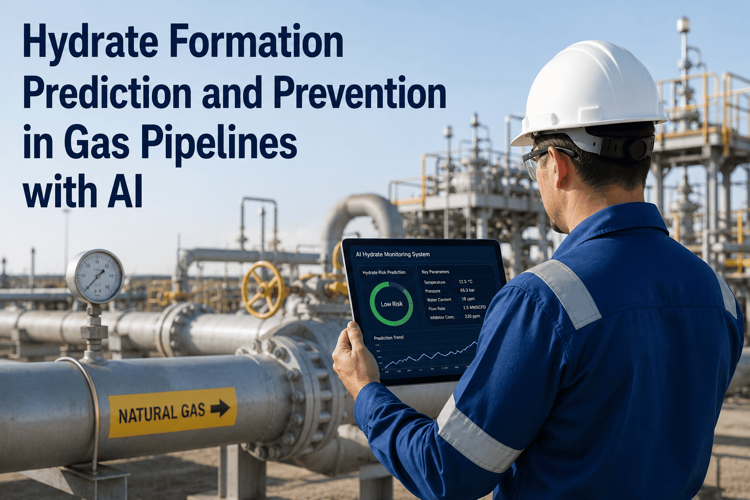
A subsea gas pipeline sitting at 3,000 psi and 4°C on the seafloor is living inside a hydrate formation window whether anyone is watching the number or not — and for decades, the only way to know how close to that line the system actually was ran through a lab technician correlating a spot-check gas sample against a chart. Gas hydrates are ice-like solid crystals that form when light hydrocarbon molecules get trapped inside a cage of water molecules under high pressure and low temperature, and once enough of them form together, they behave exactly like a plug of ice sitting inside a pipe that was never designed to be pigged clear of solid ice. iFactory's flow assurance monitoring turns that spot-check into a continuous, real-time subcooling calculation, so the operating team knows the actual margin to hydrate formation at every point along the line, not just the margin implied by yesterday's lab result.
How Close Is Your Gas Really Running to the Hydrate Line?
Hydrate formation is a pressure-temperature problem first and a chemistry problem second. AI models the equilibrium curve continuously against live process data, so subcooling margin — not a periodic lab sample — becomes the number that drives methanol and glycol injection.
What Actually Happens Inside a Hydrate-Forming Line
Gas hydrates are not a residue or a scale — they are a distinct solid crystalline phase, water molecules locked into a cage structure around a trapped gas molecule, and once formed they hold together with enough mechanical strength to fully occlude a pipe. Any wet gas stream carrying free water or water vapor is a candidate, and the two variables that decide whether the crystal actually forms are pressure and temperature: raise the pressure, lower the temperature, and the system moves toward the hydrate stability region. At roughly 100 bara, hydrates can begin forming at temperatures as high as 20°C; push the pressure up toward 400 bara and that threshold climbs to around 30°C, which is why high-pressure gas gathering systems and deepwater flowlines are structurally the highest-risk environments in the industry, not an edge case.
The Hydrate Equilibrium Curve
A pressure-temperature boundary specific to a given gas composition and water content. Operating conditions on the high-pressure, low-temperature side of that curve sit inside the hydrate-stable region; everything on the other side is safe from a thermodynamic standpoint.
Subcooling Margin
The temperature difference between the actual operating temperature and the hydrate equilibrium temperature at that same pressure. A shrinking margin — not a fixed alarm threshold — is the real early-warning signal flow assurance engineers are trying to track.
Induction Time
The delay between a system entering the hydrate-stable region and visible crystal growth actually beginning. Conditions can sit inside the risk zone for a period before a plug forms, which is exactly the window continuous monitoring is built to catch.
The Four Inputs an AI Model Actually Needs
A rule-of-thumb hydrate temperature — the commonly cited figure that methane hydrates can begin forming near 4°C at pressures as low as 170 psig — is a useful mental anchor, but it is nowhere near precise enough to set an actual injection rate against, because real production gas is never pure methane and real pipelines never hold one steady pressure along their length. A continuous prediction model instead recalculates the equilibrium curve against the actual, current values of four variables, updating the subcooling margin every time any one of them shifts.
Line Temperature
Measured at multiple points along the pipeline, not just at the wellhead, since seafloor and buried-line temperatures vary significantly from the inlet condition.
Line Pressure
Both operating pressure and pressure drop profile along the line, since the equilibrium temperature shifts meaningfully with pressure at every point.
Gas Composition
Specific gravity and heavier-component content change the equilibrium curve itself — the same temperature and pressure can be safe for one gas stream and inside the hydrate region for another.
Water Content
Free water availability, water cut trends, and dew point data determine whether there is actually enough water present for a hydrate to form in the first place.
Thermodynamic vs. Kinetic Inhibitors: Two Different Strategies
Not every hydrate inhibitor works the same way, and dosing the wrong one — or the right one at the wrong rate — either wastes chemical spend or leaves real risk on the table. Thermodynamic inhibitors physically shift the equilibrium curve itself, while kinetic and anti-agglomerant chemistries take a different approach entirely, working within the hydrate-stable region rather than trying to move out of it.
Methanol
The most widely used thermodynamic inhibitor, effective at suppressing the hydrate point by tens of degrees at typical injection rates and well suited to systems where the methanol cannot be economically recovered and recycled.
MEG (Monoethylene Glycol)
A higher-boiling-point thermodynamic inhibitor favored in systems with onshore or platform regeneration infrastructure, since MEG can be reclaimed and reinjected rather than consumed on a single pass.
Kinetic / Anti-Agglomerant Inhibitors
Low-dose chemistries that delay crystal growth or keep small hydrate particles dispersed as a flowable slurry rather than preventing formation outright, typically dosed at a fraction of the volume required for methanol or MEG.
Manual Sampling vs. Continuous Prediction
Most flow assurance programs still run on a combination of periodic gas sampling, lab-derived equilibrium curves, and a fixed injection rate set conservatively enough to cover the worst case the engineer can imagine. That approach is not wrong, exactly — it is simply built around the data that was available at the time it was designed, and it treats a continuously shifting risk as if it were a fixed number.
| Dimension | Manual Sampling Approach | Continuous AI Prediction |
|---|---|---|
| Update Frequency | Periodic — daily, weekly, or per lab turnaround | Continuous, recalculated as conditions change |
| Injection Rate Basis | Fixed rate set for worst-case conditions | Dynamic rate matched to live subcooling margin |
| Composition Sensitivity | Assumes composition is stable between samples | Recalculates equilibrium curve as composition shifts |
| Chemical Spend | Typically overdosed for safety margin | Right-sized to actual required suppression |
| Early Warning | Detected after the fact, often at a pressure drop | Flagged as the margin narrows, before formation begins |
The Cost of Getting Injection Rate Wrong in Either Direction
Hydrate management is a balance problem, not a maximize-safety-margin problem, because both sides of the dosing decision carry a real cost. Underdosing risks an actual plug, which can take a line out of service for days while a remediation approach — controlled depressurization, direct heating, or chemical dissolution — is planned and executed, often under real safety constraints since an uncontrolled release of a pressurized plug is itself hazardous. Overdosing is the quieter cost: continuous excess methanol or glycol spend across a field with dozens of wells adds up to a meaningful operating expense over a year, and excess methanol carried downstream can complicate gas processing and increase regeneration load on glycol dehydration units.
Stop Choosing Between Overdosing and Risking a Plug
iFactory recalculates required inhibitor volume continuously against live subcooling margin, so injection rate tracks actual risk instead of a fixed worst-case number carried for years without review.
A Composite Scenario: The Gathering Line That Kept Losing a Shift a Month
A mid-continent gas gatherer operating a network of high-pressure lines feeding a central compressor station had, for years, run methanol injection at a single conservative rate set once during original design and rarely revisited. The rate was based on the coldest expected ambient winter condition and the richest gas composition the field was expected to produce, which meant that for most of the year, on most of the wells, the system was significantly overdosed relative to actual risk. It was also, on the coldest days combined with a temporary spike in produced water from a newly completed well, occasionally underdosed — and the gathering system lost roughly one shift a month to a suspected hydrate restriction somewhere in the network, without ever being able to pinpoint exactly where.
When the operator deployed continuous subcooling monitoring across the gathering system, the picture that emerged was sharper than anyone expected. Two specific well laterals, both tied into a section of line with unusually low burial depth and higher exposure to ambient temperature swings, accounted for nearly all of the near-miss subcooling events — while the rest of the network was running with a comfortable, unnecessary margin nearly every day of the year. Injection was re-tuned lateral by lateral rather than field-wide: the two exposed laterals got a higher, temperature-responsive dose during cold snaps, and the rest of the field's dose rate came down significantly with no increase in risk. The monthly restriction events stopped within the first full winter under the new dosing profile, and total methanol spend across the field dropped by a meaningful double-digit percentage even after accounting for the higher dose on the two at-risk laterals. The operator's flow assurance engineer put it simply afterward: the field had never actually had a hydrate problem — it had a data problem that happened to look like a hydrate problem two laterals at a time.
Rolling Out Continuous Hydrate Monitoring
Moving from a fixed conservative dose rate to a continuously optimized one is not a single switch-flip — it is a staged process that builds confidence in the model before dose rates actually change in the field, since an injection rate change on a live pipeline is not something to get wrong.
Baseline Data Integration
Connect live temperature, pressure, and available gas composition data across the target lines, and validate the equilibrium curve calculation against historical lab samples before trusting it in real time.
Shadow Monitoring
Run the continuous subcooling calculation alongside the existing fixed dose rate without changing injection, comparing the model's flagged risk periods against actual field observations.
Segment-Level Dose Tuning
Adjust injection rate by line segment or well lateral rather than field-wide, starting with the segments showing the clearest gap between fixed-rate assumptions and live subcooling data.
Full Dynamic Dosing
Move injection control to continuous, model-driven rates across the full network, with alerting for any segment where subcooling margin narrows faster than the model expects.
Common Mistakes When Building a Hydrate Prediction Program
Treating One Fixed Rate as Permanent
A dose rate set once during design and never revisited drifts further from actual field conditions every year as gas composition, water cut, and production rates change.
Ignoring Gas Composition Drift
Focusing only on temperature and pressure while assuming composition is stable misses the fact that a heavier or leaner gas stream shifts the equilibrium curve itself, not just the operating point.
No Segment-Level Visibility
Monitoring only at the wellhead or the compressor station misses the exact points along a long gathering line where burial depth and ambient exposure actually create the highest risk.
Frequently Asked Questions
What is subcooling margin and why does it matter more than a single hydrate temperature?
Subcooling margin is the gap between the actual operating temperature and the hydrate equilibrium temperature at the current pressure and gas composition, and it matters more than any single fixed threshold because the equilibrium temperature itself moves as pressure and composition change. A pipeline can be perfectly safe at a given temperature under one set of conditions and inside the hydrate-stable region at that exact same temperature under slightly different ones, which is why a continuously recalculated margin is the number worth tracking rather than a static alarm point. Visit support to see how the margin is calculated from your specific process data.
Can AI actually predict hydrate formation before it happens, or only detect it afterward?
The value of continuous prediction is specifically in the before — by recalculating the equilibrium curve and subcooling margin against live process data, the model flags a narrowing margin while there is still time to adjust inhibitor dosing, rather than waiting for a pressure drop or flow restriction that signals a plug has already begun forming. Induction time between entering the hydrate-stable region and visible crystal growth gives a real window to act, and that window is exactly what a fixed-schedule sampling approach cannot see. Book a demo to see this modeled against a real pipeline profile.
How much can methanol or MEG spend actually be reduced with continuous dosing?
The reduction depends heavily on how conservative the existing fixed rate was to begin with, but fields running a single worst-case dose rate across a network with meaningfully different exposure by segment or lateral tend to find the largest opportunity, since most of the network was likely overdosed most of the time to cover a small number of higher-risk points. The right way to measure the opportunity is establishing an accurate segment-by-segment baseline first rather than assuming a fixed percentage savings applies everywhere.
What data does a facility need before it can run continuous hydrate prediction?
At minimum, a usable model needs live or near-live temperature and pressure data at relevant points along the pipeline, a reasonably current gas composition profile, and some visibility into water content or water cut trends, since all four of those variables feed the equilibrium curve calculation. Facilities without full instrumentation coverage today are not excluded — a phased rollout that starts with the best-instrumented segments and expands from there is a normal way to build toward full network coverage.
Is kinetic inhibitor dosing handled the same way as methanol or MEG dosing?
Kinetic and anti-agglomerant inhibitors work on a fundamentally different mechanism than thermodynamic inhibitors — they don't shift the equilibrium curve the way methanol or MEG does, so a subcooling-margin-based dosing model needs to account for which inhibitor class is actually in use before recommending a rate. A program built around thermodynamic inhibitor dosing logic should not be applied unmodified to a kinetic chemistry without reviewing that distinction first. Contact support to review which model fits your current inhibitor program.
Know Your Subcooling Margin Before the Line Does
iFactory turns live temperature, pressure, and composition data into a continuous hydrate risk picture — so injection rate is driven by what's actually happening in the line, not a number set once and carried for years.