A steel plant already measures its carbon. Fuel burned, power drawn, scrap charged, heats tapped, tonnes shipped — the numbers exist, scattered across the control room, the energy meters, the lab and the finance system. The problem is not that the data is missing. It is that the EU border mechanism asks for a different cut of the same plant than the one your sustainability team built. Exporters who want to see both cuts drawn from a single model can walk through a unified emissions data layer on real heat records.
One Plant, Two Emissions Cuts — Built From The Same Data
iFactory AI joins Scope 1, 2 and 3 corporate accounting with CBAM's installation and good-level embedded emissions, so your declaration runs on verified actuals instead of punitive default values.
Why The Data You Have Is Not The Data CBAM Wants
Most steel producers that report to the EU already run a corporate carbon inventory. It follows the familiar three-scope split and it answers the question an investor asks: how much carbon does the whole company emit in a year?
The border mechanism asks a narrower, sharper question: how much carbon is embedded in this specific tonne of hot-rolled coil crossing into the EU, measured the EU way, and can an accredited verifier stand behind the number? Those are not the same question, and the same database rarely answers both without rework.
Where The Two Models Pull Apart
The gap between a Scope-based inventory and a CBAM-ready dataset is not a matter of effort. It is structural — different boundaries, different inclusions, a different unit of account. The matrix below lines them up side by side; scroll it on a narrow screen.
| Dimension | Scope 1 / 2 / 3 inventory | CBAM cut for steel |
|---|---|---|
| Unit of account | The whole company or a site, per year | Each imported good, per tonne |
| Electricity | Scope 2, always counted | Excluded from definitive-phase steel embedded emissions |
| Upstream inputs | Broad Scope 3, estimated | Specific precursors only, with their own embedded figure |
| Method | GHG Protocol, flexible | EU method, calculation or measurement based |
| Proof | Assurance optional in many regimes | Independent verification before the annual filing |
| Fallback | Estimates and averages accepted | Default values apply, set deliberately high |
Read the electricity row twice. A plant that routes every kilowatt-hour into its carbon story is doing right by Scope 2 — yet for steel in the definitive phase that same electricity sits outside the embedded-emissions figure. Pour it into the border number by habit and the good looks dirtier than the rules say it is.
The precursor row hides a second trap. A corporate inventory treats purchased pig iron or crude steel as a broad category of upstream carbon, often filled with an industry average. The border cut needs the embedded figure of that specific precursor, carried into the finished good. An average that was good enough for disclosure quietly inflates the number that now costs money.
So the gap is not sloppiness. Two honest, well-run reporting programmes can produce two different numbers for the same steel because they were built to answer different questions. The trouble starts only when a plant assumes one can stand in for the other.
Three Gaps That Quietly Trigger A Default
A default value is not a punishment handed down for high emissions. It is what the rules fall back to when the number cannot be trusted. Three ordinary data gaps are enough to force one, even on a clean plant.
None of these is about how much carbon the furnace releases. Each is about whether the data was joined, attributed and settled in time. That is why a plant with genuinely low emissions can still pay a high-emissions charge, and why the fix lives in the data layer rather than the melt shop.
What A Data Gap Actually Costs
When verified actual emissions are not supplied, the EU applies default values. For a coal-heavy, blast-furnace route they are set high on purpose, and Indian steel sits among the most exposed of any major exporter. The bars show an illustrative gap between a default-driven figure and a verified one, indexed to the verified case at 100.
The pattern is what matters. A number you cannot defend is scored against the worst plausible plant, and the charge is set accordingly. A verified number priced against your own furnaces can be a fraction of it, and a scrap-fed electric route lands lower still.
For an Indian exporter the stakes sharpen. The country's steel leans on coal-fed blast-furnace production, which already sits high on the emissions curve, so the gap between a default and a verified figure is wide to begin with. Leaving it unmeasured means absorbing the widest version of that gap on every tonne shipped into the EU.
See Your Own Heats Projected Into A Border-Ready Number
Book a 30-minute session and iFactory AI will take a sample of your heat and shipment records and show the Scope cut and the CBAM cut drawn from the same data.
One Data Foundation, Two Outputs
The fix is not a second reporting team. It is a single data layer that ingests the plant once and projects whatever each framework needs. The flow below runs left to right: raw sources into a unified model, then out to each output.
The value of building it this way is that nothing is reported twice from two sources that can drift apart. The corporate team and the trade team read the same underlying figures, so a question in the boardroom and a question at the border resolve to one answer rather than two that have to be reconciled later.
What Changes Once The Number Is Verified
The move from a default-driven figure to a verified one is not only a lower charge. It changes how the exporter is positioned in front of its EU buyer, who has every reason to prefer a supplier whose carbon is proven.
A lower, verified number is a commercial argument as much as a compliance one. It lets a producer hold price where a rival on defaults has to discount, and it turns years of quiet efficiency work into a figure a customer can actually see.
The Quarterly Rhythm Behind An Annual Declaration
The transitional phase, which ran to the end of 2025, asked for quarterly reports. The definitive phase replaced them with one verified declaration a year — the first, for 2026, falls due in late September 2027. That sounds like less work. It is actually more, concentrated into a single filing that now carries financial weight.
The plants that stay calm keep the old quarterly cadence as an internal rhythm, even though only one filing leaves the building. They close a clean emissions quarter every three months, so the annual declaration is an assembly job, not a year-end excavation.
The difference shows up in the verification bill. A verifier handed a year of settled, traceable data moves quickly; one handed a pile of half-matched records spends the engagement chasing gaps, and every gap is a candidate for a default. The internal quarter is cheaper long before the deadline arrives.
What A Border-Ready Data Layer Must Join
The reason this is a data-integration problem and not a spreadsheet problem is that the inputs live in systems that were never built to talk to each other. Each one holds a piece of the embedded-emissions story, and none holds the whole of it.
A spreadsheet can add these up once. It cannot keep them matched, month after month, as meters recalibrate, scrap mixes change and new precursor suppliers come on. That upkeep is the real work, and it is where a manual process slips back toward defaults without anyone deciding to.
Process And Furnace Data
Heat-level energy, fuel and timing from the control layer — the backbone of the direct figure.
Energy And Fuel Metering
Metered gas, coke and power, reconciled so combustion emissions tie out to real consumption.
Charge And Scrap Mix
The scrap share per heat, which moves the route and the number more than almost anything else.
Precursor Records
Pig iron, crude steel and other bought-in precursors, each carrying its own embedded figure into the good.
Lab And Mass Balance
Carbon content and yield checks that let the calculation close against measured chemistry.
Shipment And Tonnage
The link from production to the specific consignment that crosses the EU border.
The Levers That Matter For Indian Exporters
Two structural facts shape how much an Indian steel producer pays, and both turn on data as much as on carbon.
Where iFactory AI Fits
iFactory AI sits across the plant's existing systems and builds the unified emissions model heat by heat, so both the corporate cut and the border cut come from one audited foundation.
It is the same smart-manufacturing platform that already reads furnace, meter and quality data on the plant floor — here pointed at carbon rather than throughput. The emissions model is not a bolt-on; it rides on the data the plant is already producing every heat.
Source Joining
Control, metering, lab, precursor and shipment data are matched by heat and time into one model.
Dual Projection
The same data projects a Scope 1 / 2 / 3 ledger and a good-level border cut, each by its own rule.
Default Flagging
Any good still leaning on a default value is flagged early, while there is time to supply the actual.
Verifier Evidence
Every figure keeps its raw reading and lineage, assembled into a pack an accredited verifier can review.
A Short Data-Readiness Self-Check
Run these against your own plant before the next filing window. A no is a gap worth closing while there is still time.
Frequently Asked Questions
Does our Scope 1, 2 and 3 inventory already cover CBAM?
Not on its own. A corporate inventory answers a company-and-year question, while the border mechanism asks a good-and-tonne question measured by the EU method. The underlying plant readings overlap heavily, but the boundaries, the electricity treatment and the precursor detail differ. The efficient path is to hold the raw data once and project both cuts from it rather than running two separate programmes.
Why not just accept the default values and skip the data work?
Default values are set deliberately high, and for coal-heavy steel routes they sit well above a verified figure. Accepting them means paying as if your plant were among the dirtiest plausible, which for many Indian producers is a serious overcharge. Verified actuals are the one route to a lower number, and they depend on the data being joined and traceable. You can see the default-versus-verified gap on your own route in a short session.
Does electricity count in the steel number?
For iron and steel in the definitive phase, the embedded-emissions figure focuses on direct emissions, and electricity is treated outside it, even though power is a major input. That is a key difference from a Scope 2 inventory, where electricity is always counted. Confirm the current treatment for your specific goods, because the rules differ by product group and continue to evolve.
We report annually now, so why keep a quarterly rhythm?
Because the annual declaration is verified and financially binding, assembling a full year at the deadline is where errors and default fallbacks creep in. Closing each quarter internally keeps the data settled, so the filing is an assembly step and the verifier reviews finished work. It is a habit the definitive phase rewards even though it no longer requires the four reports.
What data do we need before we start?
The core is heat-level process data, metered energy and fuel, scrap and charge records, lab or mass-balance checks, precursor purchase details and the shipment link to each consignment. Most plants already hold these across control, lab, procurement and finance systems. The early weeks focus on matching them by heat and time so the good-level number can be built and defended.
Build The Border Number From Data You Already Have
iFactory AI joins your plant's emissions data once and projects both the Scope ledger and the CBAM cut, with the lineage a verifier needs. Book a walkthrough on your own heats.