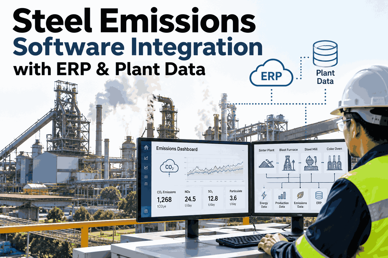
Every emissions figure a steel plant reports comes down to one line of arithmetic: activity data multiplied by an emission factor. The factor is a lookup anyone can maintain. The activity data is the hard part — fuel flows, tonnage, purchased power and material volumes that already exist, scattered across the historian, the MES and the ERP. Integration is the work of wiring the system that calculates emissions to the systems that already measure the activity, so each number computes from its own source instead of being typed into a spreadsheet once a quarter. Teams that want this mapped on their own stack can book a working session.
Wire the Emissions Number to the Systems That Already Measure It
iFactory AI connects your carbon calculation to SAP, Oracle and the plant historian, so Scope 1, 2 and 3 compute from live activity data and trace back to the meter that produced them.
The Whole Problem, in One Equation
Carbon accounting under the GHG Protocol is deliberately simple arithmetic. Emissions equal activity data times an emission factor. Reporting gets hard not because the maths is hard, but because one of the two inputs is scattered across systems that were never built to talk to each other. Steel sits at roughly seven percent of global carbon emissions, so the number matters, and so does being able to prove it.
Where Each Emissions Number Actually Lives
Nothing on this page needs to be invented — the numbers already exist inside systems the plant runs every day. The real job is knowing which system owns each input and connecting to it at the right tempo. Engineers can see the connection map for their own environment.
| Emissions input | Where it lives | Scope | How it connects |
|---|---|---|---|
| Fuel & gas flow — coke oven, blast furnace, reheat | SCADA / historian (Level 2) | Scope 1 | OPC-UA / historian connector |
| Process rate & charge records | MES (Level 3) | Scope 1 | REST API |
| Steel tonnage produced | MES / production orders | Intensity base | REST / scheduled sync |
| Purchased electricity & steam | ERP utility ledger / meters | Scope 2 | Meter feed + ERP records |
| Raw material & alloy volumes | ERP procurement — SAP MM / Oracle | Scope 3 | Scheduled ERP export |
| Inbound & outbound freight | ERP logistics records | Scope 3 | Scheduled ERP export |
| Emission factors | Factor reference library | All scopes | Maintained lookup |
Three Systems, Three Different Clocks
The reason this data never merged on its own is tempo. Each system reports at a different speed, and a quarterly report and a live dashboard end up disagreeing simply because they sampled different moments. An integration layer absorbs the mismatch so both draw from the same source.
The Hidden Cost of the Quarterly Scramble
Before any of this is wired together, the footprint is usually rebuilt by hand at the end of each reporting period. It works, but it carries a cost that rarely shows up on a budget line — the cost of a number nobody can quite stand behind.
None of that is a failure of effort. It is a failure of plumbing — the right numbers existing in the right systems with no wire between them and the report. That gap is what an integration closes, and it is worth seeing on a real stack rather than in the abstract.
See It Wired to Your Own SAP or Historian
Book a 30-minute session and iFactory AI will map the connection from your ERP and plant historian to a live Scope 1, 2 and 3 calculation.
The Three Connections That Do the Work
Most steel producers do not run one clean system — they run SAP alongside a historian alongside an MES, often across several sites with different plant codes. Each source needs its own handshake, and each one is read-only.
SAP
SAP PM, MM and CO/FI on ECC or S/4HANA hold procurement volumes, cost centres and utility postings. A read connection pulls the activity data behind Scope 2 and Scope 3 without touching the configuration the plant spent years building, and it works across multiple plant codes and controlling areas.
Oracle
Oracle E-Business Suite and Fusion expose the same procurement and energy records through REST services. Each material volume is mapped to the right plant, cost centre, product and period before it reaches the calculation, so the figures land where they belong.
Plant historian
OSIsoft PI, AVEVA and equivalent historians carry the real-time fuel, gas and process tags that drive Scope 1. A read-only tag subscription streams them in continuously over OPC-UA, matched to the unit that produced each reading.
What Actually Moves Across the Connection
It helps to be concrete about the data itself. The connection does not move documents or dashboards — it moves four simple kinds of record, which the calculation then assembles into an emissions figure.
Why the Spreadsheet Fails the Audit, Not the Maths
The common setup is an EHS analyst rebuilding the footprint each quarter from fuel invoices and utility bills. The arithmetic is usually right. What fails under review is provenance — no one can show which meter, which heat or which invoice a number actually came from.
Master Data: the Real Reason Integrations Stall
When an emissions integration stalls, the cause is almost never the protocol. It is that the same physical thing has a different name in every system, so the data cannot be lined up. Fixing this once is most of the work — and the part worth getting right.
One asset, three names
The reheat furnace is a tag group in the historian, a cost centre in SAP and an asset number in the MES. Until those point at one identity, its fuel and its tonnage cannot meet.
Materials that do not line up
Iron ore in the purchase ledger and the charge record in the MES often use different codes and units. The Scope 3 figure depends on reconciling them to the same quantity.
Mapped once, not every quarter
Map each source identity to a single master the first time, and every future reading lands against the right unit, product and period automatically — no monthly re-keying.
Which Source Feeds Which Scope
Each scope draws from a different corner of the plant's systems. Connecting the right source to the right scope is what turns three separate reporting exercises into one pipeline that runs itself.
CBAM and the 2026 Reporting Reality
The reason this has moved from a sustainability nicety to an operational requirement is regulation. Several frameworks now expect emissions that are not just reported, but defensible — and they expect them more often than once a year.
CBAM
The EU Carbon Border Adjustment Mechanism asks importers of covered steel to report embedded emissions on a quarterly basis, moving toward a financial obligation. Primary, source-backed data beats default values here.
CDP & investors
Annual environmental disclosure increasingly expects audited, traceable figures rather than estimates. Buyers of low-carbon steel ask for the same evidence on a per-product basis.
National rules
Climate disclosure requirements in several markets push for consistent, repeatable Scope 1 and 2 reporting that stands up to external review, period after period.
From Meter Reading to Disclosure, Without Losing the Thread
The value of integration is not a prettier dashboard. It is a number that can defend itself. Each step keeps the identity of the step before it, so any reported figure can be unwound all the way back to the physical reading that started it.
A Composite Picture: One Mill, One Number
The following is an illustrative composite, not a single named site, but it mirrors how integrated producers have begun wiring CO₂ dashboards straight into ERP-SAP for real-time, department-level tracking.
Where iFactory AI Fits
Building this needs connectors, a calculation engine and discipline about provenance. iFactory AI supplies the data foundation and the calculation layer that sit between your plant systems and your carbon disclosures.
Universal Connectors
Read connections to SAP, Oracle, Dynamics and major historians over OPC-UA, MQTT and REST, across multiple sites and plant codes.
Live Activity Capture
Fuel, gas, power and tonnage stream in continuously and map to the unit and period that produced them.
Factor Library & Calc
GHG Protocol-aligned factors applied automatically, with Scope 1, 2 and 3 computed per tonne and per period.
Traceable Reporting
Every figure keeps its source, so CBAM, CDP and internal reports pull from one audited chain.
An Integration-Readiness Shortlist
A connection goes faster when a few decisions are made first. None of these need new instruments — they are about knowing what you already have and how it should line up.
Who Actually Uses the Connected Number
Once the pipeline runs, the same figure gets used by more people than the original spreadsheet ever reached, because each team can now trust it enough to build on it rather than re-deriving their own version.
EHS & sustainability
Files the quarterly and annual disclosures from a number that is already reconciled, instead of assembling one from invoices under deadline pressure.
Plant & process engineers
See emissions per tonne alongside the operating data they already watch, so an efficiency change can be weighed on carbon as well as cost.
Finance & procurement
Use the same Scope 3 figures when weighing supplier contracts or a CBAM exposure, drawing on the ERP data they already own rather than a separate estimate.
Frequently Asked Questions
Does iFactory AI replace our ERP or emissions system?
No. iFactory AI is an integration and calculation layer, not a replacement. It reads activity data from SAP, Oracle or the historian and leaves those systems exactly as they are. You keep the ERP configuration and control systems you already run, and the emissions calculation simply draws from them. For teams wanting to see the mapping on their own stack, support can walk through the setup.
Which ERP and historian systems can connect?
On the ERP side, SAP ECC and S/4HANA with PM, MM and CO/FI, Oracle E-Business Suite and Fusion, and Microsoft Dynamics. On the plant side, OSIsoft PI, AVEVA and most OPC-UA or MQTT historians. Connections are read-only by default, so nothing writes back into the ledger or the control layer. New sources can be added as the plant grows.
How does integration help with CBAM and audits?
Because every reported figure keeps the source reading it came from, a CBAM filing or an audit can be traced from the disclosed tonne of CO₂ back to the meter, heat or invoice behind it. That provenance is the part a reviewer asks for, and the part a quarterly spreadsheet cannot supply. You can walk the traceability chain on your own data in a short session.
Is the activity data accurate enough to report?
The data is as accurate as the instruments already feeding your plant systems — the same meters and records you run on today. Integration adds reconciliation: where a feed is missing or a reading drifts, the gap is flagged rather than quietly filled with an estimate. That is usually more defensible than a hand-keyed spreadsheet built from monthly bills.
How long before the numbers are reliable?
A first calculation of Scope 1 and 2 can run inside the rollout window, since that data is already metered. Scope 3 firms up over the first few reporting periods as procurement records are mapped and suppliers publish product-level factors. The pipeline is designed to accept better factors as they arrive, without being rebuilt each time.
Compute the Number Once, Trace It Forever
iFactory AI connects your ERP and plant data to a live Scope 1, 2 and 3 calculation that any auditor can follow. Book a walkthrough to see it running on your own systems.