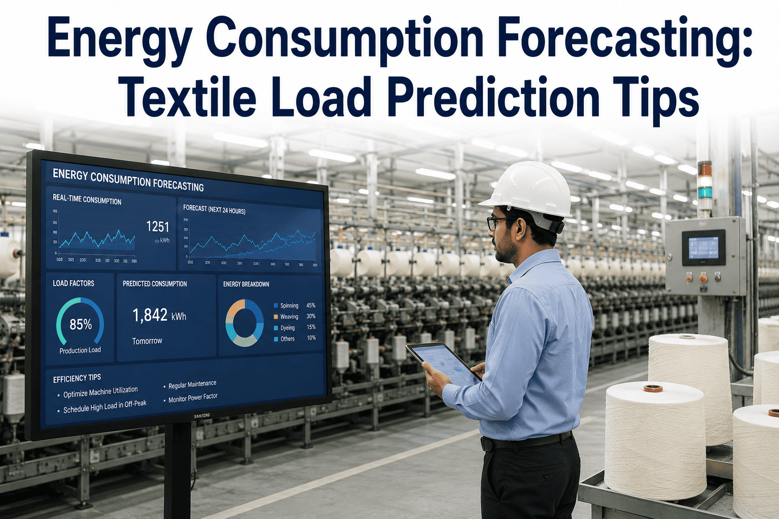
A dyeing house running three shifts can watch its electricity bill swing by thirty percent month to month with no obvious pattern, because nobody connected the production schedule to the load curve until the invoice arrived. Energy consumption forecasting closes that gap by predicting, in advance, how much power a textile plant will draw hour by hour based on what is actually scheduled to run, so procurement, maintenance, and shift planning can all work from the same number instead of finding out together at month end. The plants that get this right are not buying better electricity — they are simply the first to know what they are about to use, which turns energy from an unpredictable cost line into a plannable one, and that shift alone changes how procurement, maintenance, and shift planning treat every subsequent billing cycle. Book a demo to see how forecasting connects to your existing production schedule.
Your Production Schedule Already Tells You Your Energy Bill — If Anyone Reads It
Compressors, dyeing machines, stenters, and boilers each carry a predictable load signature. Forecasting stitches those signatures to your actual production plan so you see the electricity draw before it happens, not after it is billed, giving procurement and planning a shared, forward-looking number instead of a rear-view one.
Most Textile Plants Plan Production and Plan Energy Separately
Production scheduling lives with the planning team, and the electricity bill lands with finance a month later, and by the time anyone connects the two the shift is long finished and the demand charge is already locked in. This separation is the actual root cause behind most energy cost surprises in textile manufacturing, not equipment inefficiency or tariff structure. A dyeing machine and a stenter drawing peak load in the same thirty-minute window can push a plant into a higher demand tariff bracket for the entire billing cycle, and that decision gets made unknowingly every time two high-draw processes happen to overlap on the floor. Ask most plant managers what tomorrow's peak demand will be and the honest answer is that nobody knows until it has already happened, because the tools tracking production and the tools tracking energy were never designed to talk to each other in the first place.
The consequence compounds over a full financial year. A single avoidable demand spike costs one month's penalty, but the same blind overlap recurring across twelve billing cycles becomes a permanent, invisible tax on production — one that shows up on the profit and loss statement as a vague "utilities" line rather than being traced back to a schedule that could have been rearranged for free. Energy teams end up managing the bill after the fact through tariff renegotiation and power-factor correction, both of which are worth doing but neither of which addresses the actual cause: nobody forecasted the load before it happened.
Energy Consumption Breaks Down Very Differently Across a Textile Plant
A composite mill running spinning, weaving, dyeing, and finishing under one roof does not draw power evenly across those stages, and treating the plant as a single undifferentiated load is one of the fastest ways to build a forecast that misses on the days that matter most. Dyeing and finishing are thermal-heavy and dominate both electrical and steam demand, spinning draws steadily but predictably across long production runs, and weaving sits in between with load tied closely to loom count and shuttle speed rather than fabric type. Forecasting that treats these stages separately, using their own load signatures, consistently outperforms a single blended model applied across the whole facility, because averaging a steady spinning load together with a spiky dyeing load smooths out exactly the peaks a forecast needs to catch.
This is also why a plant-wide average consumption figure, the kind most utilities report on a monthly statement, tells you almost nothing useful about where to focus improvement effort. Two mills with identical total monthly consumption can have completely different risk profiles — one carrying its load steadily across spinning and weaving, the other concentrating a large share into a handful of dyeing batches — and only a process-level breakdown reveals which mill actually needs peak-management attention first.
Three Ways to Predict Your Load, Ranked by What They Actually Need
Not every plant needs the most sophisticated forecasting method available, and choosing the wrong tier is as costly as choosing none at all — a statistical model applied to a plant with constantly shifting product mix will underperform, while a full machine-learning deployment on a stable single-product line is more infrastructure than the problem requires. The right starting point depends less on plant size and more on how variable your product mix and schedule actually are week to week, which is worth being honest about before committing budget to a tier the operation does not need yet. The table below lays out what each method needs as input and where it tends to break down, scrollable on smaller screens.
| Method | Input Needed | Typical Accuracy | Best Fit |
|---|---|---|---|
| Historical averaging | Past 12 months billing data | 60–70% | Stable, single-product lines |
| Statistical regression | Production volume + weather + shift data | 75–85% | Plants with predictable seasonality |
| Machine-level ML forecasting | Machine load signatures + live schedule feed | 88–95% | High-mix plants with variable product runs |
| Hybrid (ML + procurement rules) | ML forecast + tariff structure + contract terms | 90–96% | Plants on demand-based or time-of-use tariffs |
Most plants do not need to pick permanently between these tiers on day one. A common and sensible path is to start with statistical regression using data already available in the billing system, prove out the value on paper within the first month, then justify the investment in machine-level sub-metering that unlocks the higher accuracy tiers once the initial forecast has already shown where the savings are concentrated.
Five Inputs That Determine Whether Your Forecast Is Useful
A forecast is only as good as the signals feeding it, and textile plants have a specific set of variables that matter far more than generic demand-forecasting inputs borrowed from other industries. Get these five right and accuracy climbs quickly; skip even one and the model will consistently miss on exactly the days that matter most, which are the high-load days when a wrong forecast costs the most. None of these five require a full plant rebuild to start capturing — most are already sitting in existing systems, just not connected to each other or to the forecasting layer that would make them useful.
See Load Prediction Run Against Your Own Machine Data
Bring a week of production schedule and machine load data. We will show you the forecast accuracy your plant would have gotten, using your own numbers rather than an industry average.
Why the Highest Fifteen Minutes of Your Month Sets the Whole Bill
Most industrial tariffs in India charge a demand component based on the highest sustained load recorded in any fifteen or thirty-minute window during the billing cycle, which means a single unlucky overlap between a dyeing batch startup and a compressor cycling on can set your demand charge for the entire month regardless of how efficiently every other hour ran. Peak demand forecasting specifically targets this window rather than average consumption, because average consumption is not what the utility bills on. A plant can run efficiently for every other hour of the month and still take a full month's demand penalty from one badly timed fifteen-minute overlap, which is exactly why average-consumption dashboards, however accurate they look on a monthly report, miss the single number that actually determines the bill.
This is also why peak forecasting has to work at machine-level resolution rather than department-level. A department-level view might show dyeing running comfortably within its usual range for the day, while the specific fifteen-minute window where two machines within that department started up simultaneously never becomes visible until the demand charge already reflects it on the following month's statement. Machine-level forecasting catches this because it tracks each unit's draw curve independently and flags the moment two curves are projected to overlap, days before the schedule that would cause it is even finalized.
A Forecast Is Only Useful If Procurement Acts On It
Plants on open-access or hybrid power contracts have a second lever forecasting unlocks: buying energy ahead of need rather than reacting to spot rates. A reliable weekly forecast lets a procurement team commit to a day-ahead or week-ahead purchase at a known rate instead of absorbing whatever the spot market charges during a high-demand window, and the savings from this alone frequently exceed the savings from load-shifting on plants with real exposure to variable power pricing. The forecast does not need to be perfect to be useful here — even a directionally correct week-ahead estimate is enough for procurement to avoid the worst-priced hours, because the cost of being slightly wrong on a locked-in purchase is almost always lower than the cost of being caught unhedged during a demand spike.
The same forecast also strengthens the plant's negotiating position at contract renewal. A procurement team that can show a utility or open-access supplier a documented, data-backed consumption pattern is in a materially stronger position to negotiate favorable tariff slabs than one relying on rough annual estimates, since suppliers price risk into contracts and a predictable buyer is a lower-risk buyer by definition.
What a Forecasting Rollout Actually Looks Like
Forecasting does not require ripping out existing metering or waiting for a full IoT retrofit. Most plants start with the meters and schedule data they already have, and expand machine-level granularity over subsequent phases as the value becomes clear from the first rollout. This phased approach matters because it lets the team validate the forecast against real billing cycles before committing further budget, rather than betting the entire investment on a single big-bang deployment that has to be right on the first attempt.
Common Questions on Energy Forecasting for Textile Plants
Turn Your Production Schedule Into an Energy Forecast
iFactory connects your existing schedule and meter data to a working load forecast in weeks, not quarters. See your own numbers before you commit to anything.