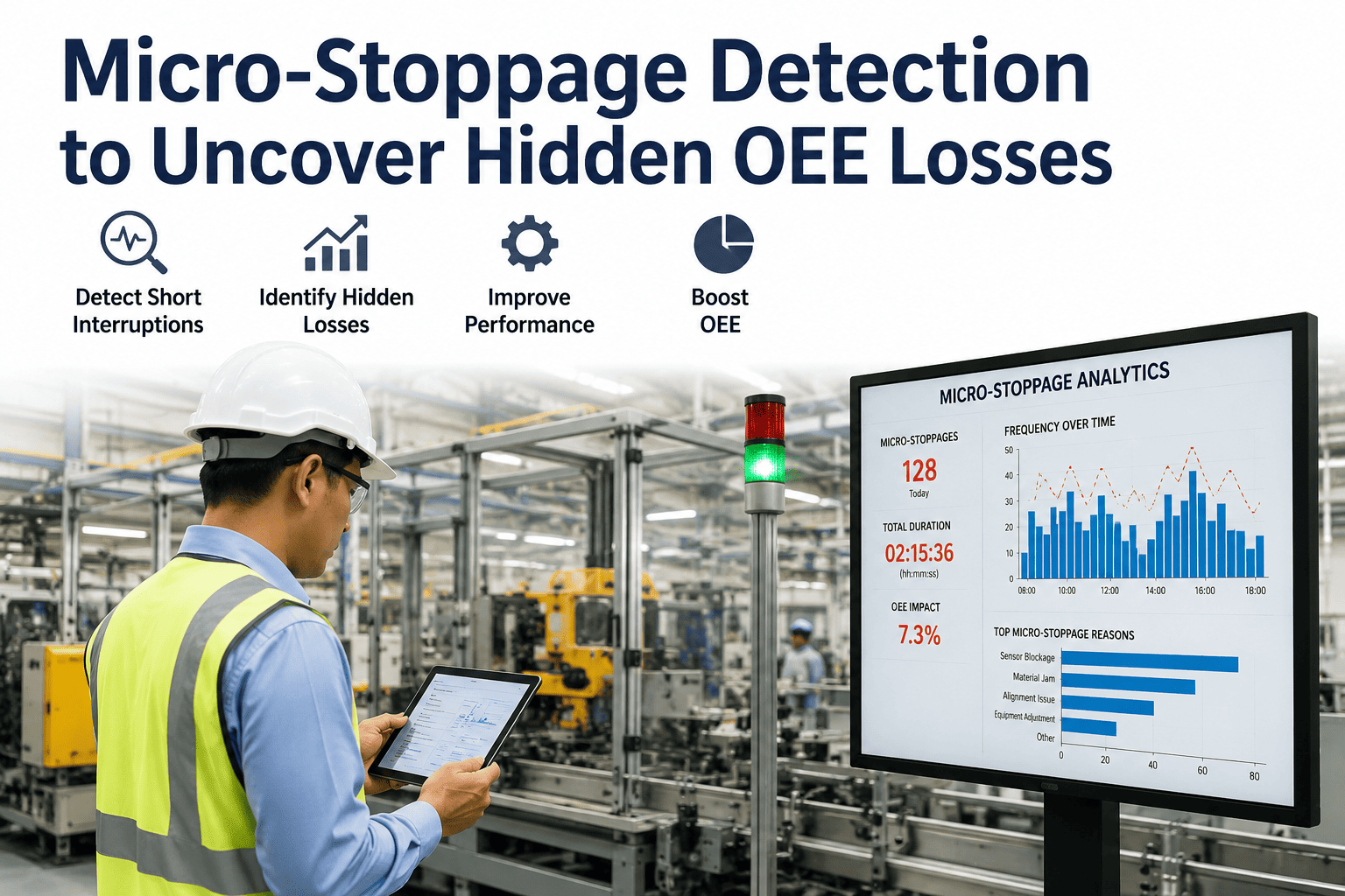
Your MES says the line ran 7.4 hours out of an 8-hour shift. Your operators logged 22 minutes of downtime. And yet the shift produced 11% below target. That missing 11% did not disappear into thin air — it drained out of the line in fragments of 2, 3, 4, and 6 seconds, hundreds of times over, in stops so brief that no operator was going to walk to the terminal to log them and no legacy OEE system was designed to catch them. This is the anatomy of a micro-stoppage problem, and it is the single most under-diagnosed source of OEE loss in discrete manufacturing today. If you want to see the losses your current system is missing, book a diagnostic walkthrough with the iFactory team.
Diagnostic Guide · OEE & Production Optimization
Micro-Stoppage Detection: Finding the OEE Losses That Never Reach Your Dashboard
A production manager's diagnostic playbook for detecting, quantifying, and eliminating the 1–5 second stops that consume 8–15 percentage points of OEE — invisible to operator logs, invisible to legacy MES, but not invisible to modern edge-AI monitoring.
8–15%
Typical OEE loss hidden in micro-stops on high-cycle discrete lines
<20%
Of sub-60-second stops that operators actually log manually
2–5 sec
Duration band where detection systems fail — and losses compound fastest
33%
Cycle performance loss from a single 4-sec stop on a 12-sec cycle
The Symptom Every CI Lead Recognises
Your Numbers Don't Reconcile — and That Gap Has a Name
What the log says
Availability 92.5%. Logged downtime events: 6 stops, 22 minutes total. Every event has a reason code. Every event was closed by an operator. The audit trail is clean.
What the throughput says
Line ran at an average 47 parts/min against a rated ideal of 60 parts/min. That is a Performance rate of 78%. Multiply by 92.5% Availability and 99% Quality — OEE lands at 71.5%.
What management asked
"If Availability is 92.5% and Quality is 99%, why is our OEE stuck at 71.5% when the industry benchmark for our line type is 85%?" You cannot answer. Your data cannot answer. The gap sits inside Performance, and Performance is a residual — a calculation, not an observation.
What is actually happening
Between the six logged downtime events, the line stopped an additional 340+ times for durations between 1.8 and 8.2 seconds each. Total accumulated loss: 47 minutes. None of it appears in any log. All of it appears in the Performance number as a mystery.
Definition Layer
Micro-Stoppage, Short Stop, Downtime — The Duration Bands That Matter
The Six Big Losses framework groups all interruptions under two headings — "breakdowns" (Availability loss) and "minor stops and reduced speed" (Performance loss). That grouping was invented in an era when human observation was the primary detection method. Modern lines cycle faster than humans can classify events. Precise duration bands are now the operational language of loss.
| Duration Band | Category | How It Reaches the OEE Formula | Typical Root Causes | Detection Difficulty |
|---|---|---|---|---|
| 0.5–2 seconds | Cycle deviation | Performance loss (invisible) | Sensor debounce, minor product variation, servo settling | Very Hard |
| 2–10 seconds | Micro-stoppage | Performance loss (invisible) | Jam clearing, misfeed, part orientation, gate cycling | Hard |
| 10–60 seconds | Short stop | Performance loss (partial) | Operator intervention, adjustment, minor reject clearance | Medium |
| 1–5 minutes | Small downtime | Availability loss (usually logged) | Material replenishment, tool change, quality check | Easy |
| 5+ minutes | Downtime | Availability loss (always logged) | Breakdown, changeover, planned stop | Trivial |
The 2–10 second band is where the losses hide. Operators will not log it. Legacy MES cannot see it. And this band is where a modern high-speed line loses more OEE than in any other category — including breakdowns.
The Compounding Arithmetic
Why Small Stops Produce Big Losses
The intuition that a 3-second stop is a trivial event is mathematically wrong on any line cycling faster than about 30 parts per minute. The loss is not the stop duration — it is the stop duration expressed as a fraction of the cycle time, multiplied by frequency.
01
Cycle-relative loss
A 4-second stop on a 12-second cycle is a 33% performance loss on that unit. On a 60-second cycle, the same 4-second stop is a 6.7% loss. The faster the line, the more damage each micro-stop does.
02
Frequency compounding
A packaging line running 60 cycles/min with 2 micro-stops per minute at 3 seconds each loses 6 seconds of every 60. That is a 10% Performance loss — every minute, every hour, every shift.
03
Cascading downstream
A 3-second stop upstream of a buffer smaller than 3 seconds of accumulation propagates to the entire line. One station's micro-stop becomes every station's Performance loss.
04
Recovery-time tax
Every micro-stop carries a recovery cost — servos ramping back up, product back-pressure clearing, sensors re-arming. A 3-second stop often produces 5 seconds of below-rated output. The visible stop is only the first half of the loss.
Worked example — automotive component line
Rated 45 parts/min. Actual observed 38 parts/min. Operators log 4 stops averaging 4 minutes each per shift — 16 minutes logged, 448 minutes running. Legacy OEE reports Availability 96.6%, Performance 84.4%, OEE roughly 80%. Edge-AI monitoring later reveals 187 micro-stops averaging 3.6 seconds per shift — 11.2 minutes of hidden loss. Once corrected, the Performance number is not a mystery: 78% of the Performance gap is now traceable to five root causes, four of which are fixable with adjustments costing under $2,000 total.
See Your Hidden Losses in 14 Days
Most Plants Discover 8–12 Points of Recoverable OEE in Their First Diagnostic Run
iFactory's micro-stoppage detection module deploys as an edge-AI layer that sits alongside your existing MES — no rip-and-replace. The first 14 days of data typically reveal more actionable loss than the prior 12 months of OEE reports combined.
Detection Physics
The Four Detection Methods — and Why Only One Works Below 5 Seconds
The reason legacy OEE software misses micro-stoppages is not a software problem. It is a signal-acquisition problem. If your input data has a resolution of 30 seconds, no dashboard on top of it can report events shorter than 30 seconds. The four detection methods in production use today have very different resolution floors.
Method 01
Manual Operator Logging
Practical resolution60–120 sec
The operator sees a stop, walks to the HMI or Andon terminal, selects a reason code, resumes the line. Human latency plus classification effort plus willingness-to-log means anything under a minute is systemically under-reported.
VerdictUnusable for micro-stop detection. Reserve for reason-code enrichment on longer events.
Method 02
MES / PLC Tag Polling
Practical resolution10–30 sec
Most MES platforms poll a "machine running" tag every 5–15 seconds. Between polls, the machine could have stopped and restarted three times — the MES sees a continuous run. Even with faster polling, the tag itself is a state flag with no duration precision.
VerdictCatches short stops above the polling interval. Blind to true micro-stops. Under-reports Performance loss by design.
Method 03
Cycle-Time Variance Analysis
Practical resolution1–3 sec
Instead of tracking "running vs stopped," this method timestamps each part-complete pulse and calculates cycle-to-cycle deviation from the ideal. Any cycle taking more than the ideal cycle time plus a variance threshold is flagged as containing a micro-stop.
VerdictDetects micro-stops but cannot classify them. Tells you when losses happen, not why.
Method 04
Edge-AI Vision + Sensor Fusion
Practical resolution0.5–1 sec
A local edge device runs a trained vision model on the line camera feed and fuses it with high-frequency PLC signals and photoelectric sensor states. It detects that motion stopped, classifies the cause using visual context, and time-stamps to sub-second precision — all without touching the MES.
VerdictThe only method that detects and classifies micro-stops with the resolution needed to build a defensible Pareto.
Prioritization Framework
Which Micro-Stops to Fix First — a Loss-Weighted Pareto
Detecting 400 micro-stops per shift is useless if the response is to try to fix 400 things. The correct output is a loss-weighted Pareto that ranks micro-stop causes by their total time contribution, not their event count. A cause that fires 3 times per shift for 12 seconds each is a bigger target than one that fires 40 times for 1 second each — even though the event count would say the opposite.
Loss Weight = Event Frequency × Mean Duration × Downstream Impact Factor
Downstream impact factor ranges from 1.0 (bottleneck station — every second lost is a shift second lost) to 0.2 (non-bottleneck with sufficient buffer — losses are absorbed). Applying this weighting typically reduces a 40-cause Pareto to 5–7 causes that account for 80% of recoverable loss.
High frequency · Short duration
Sensor debounce, part orientation micro-adjustments, servo settling. Fix with mechanical tuning, sensor placement, or firmware timing.
Action: engineering adjustment
High frequency · Long duration
The most damaging quadrant. Jam clearing on a chronic feed issue, repeated changeover-adjacent stops. Usually solvable with SMED or a mechanical redesign.
Action: root-cause project
Low frequency · Short duration
Random single-event stops. Typically not worth targeted action — they will be reduced by fixing higher-quadrant causes upstream.
Action: monitor
Low frequency · Long duration
Rare but expensive events — likely already visible in your Availability logs. Handle through the standard reliability process.
Action: reliability engineering
Implementation Roadmap
From Zero to Loss-Weighted Pareto in 6 Weeks
Week 1–2
Baseline & Instrument
Install edge devices on the target line. Configure ideal cycle time, variance threshold, and camera fields of view. Run in shadow mode — collect data alongside existing MES with no changes to operator workflow.
Week 3
Classify & Validate
Train the classification model on the first fortnight of events. Have production supervisors validate the top 20 event types against operator knowledge. Adjust classification confidence thresholds.
Week 4
Build the Loss-Weighted Pareto
Apply frequency × duration × downstream impact weighting. Identify the top 5 causes accounting for approximately 80% of recoverable loss. Present findings to production leadership.
Week 5–6
Countermeasures & Verification
Deploy engineering fixes, SMED adjustments, or operator training against the top causes. Verify improvement in the same detection layer — no reliance on before/after operator memory or MES estimates.
KPI Reference
The Metrics That Prove You Actually Reduced Micro-Stops
Micro-Stop Frequency
Track weekly
Count of detected stops between 2 and 60 seconds, per shift, per line. The leading indicator — falls before OEE rises because effort precedes result.
Mean Time Between Micro-Stops (MTBMS)
Trend upward
Inverse of frequency, expressed in the operator's language. "We used to stop every 90 seconds — now we stop every 4 minutes" is a sentence a plant manager can defend to executives.
Hidden Performance Loss
Below 2%
Percentage of available production time consumed by unlogged sub-60-second stops. Starts at 8–15% on most lines. Target of <2% is world-class.
Pareto Concentration Ratio
Above 75%
Percentage of total micro-stop time attributable to the top 5 causes. High concentration means countermeasure work will have high leverage. Low concentration means the losses are diffuse and harder to attack.
Cycle-Time Variance
Below 8% CoV
Coefficient of variation on part-complete cycle times. A statistical proxy for micro-stop presence — even before classification, high variance signals hidden losses in the Performance calculation.
Recovery Time Multiplier
Below 1.4
Ratio of total production time lost per micro-stop to the stop duration itself. Values above 1.5 indicate significant ramp-back-up losses that a stop-count metric alone would understate.
Practitioner Perspective
“
The single biggest shift in OEE thinking over the last decade is not new dashboards or better colours on the Andon board. It is the recognition that Performance is not a residual to be tolerated — it is a measurement gap to be closed. In every plant I have walked into where OEE was stuck between 68 and 75 percent, the Availability numbers looked defensible and the Quality numbers looked defensible, and the entire missing 10 to 15 points sat inside Performance with no one able to explain it. That was not an OEE problem. That was a detection problem. Once you install a layer that can see stops shorter than an operator will log, you stop debating whether the losses are real and start debating which ones to fix first. That is a much more productive argument to have on a Monday morning.
Priya Ramanathan
Continuous Improvement Lead & Lean Six Sigma Master Black Belt · 18 years across automotive tier-1, packaging, and consumer electronics · Former OEE Program Director at a Fortune 500 CPG manufacturer
Frequently Asked
Micro-Stoppage Detection — Common Questions from Production Leaders
What is the practical difference between a micro-stoppage and downtime?
Downtime is any stop long enough that an operator will notice, respond, and typically log with a reason code — usually anything from 1 minute upward, and always anything from 5 minutes upward. A micro-stoppage is a stop shorter than the human logging threshold, generally between 2 and 60 seconds, that recovers on its own or with a trivial intervention. Because operators do not log them and legacy MES tag polling cannot resolve them, micro-stops disappear into the Performance component of the OEE formula rather than the Availability component. That is why plants with clean downtime logs and clean quality logs still report OEE that no one can fully account for. If you want to see the exact micro-stop distribution on your own line before comparing vendors, start with an iFactory diagnostic session.
Why doesn't our current OEE software catch micro-stops if we already track everything through the PLC?
Most OEE platforms subscribe to a small number of PLC tags — typically a "machine running" boolean and a part-count register — polled at intervals of 5 to 30 seconds. That polling rate defines the resolution floor of every downstream metric. If the polling interval is 10 seconds, the software cannot report events shorter than 10 seconds, no matter how sophisticated the dashboard layer looks. Additionally, a "running" tag is a state flag, not a duration measurement; the machine can stop and restart between polls and the software will see a continuous run. Detecting true micro-stops requires either high-frequency cycle-timestamp capture or an independent detection layer such as vision or sensor fusion. For a walkthrough of how iFactory's edge layer integrates alongside your existing MES without replacing it, reach out to our support team.
How much OEE loss are we actually hiding in micro-stoppages on a typical line?
The range across the plants we have measured is 4 to 18 percentage points of OEE, with a central tendency around 8 to 12 points. High-cycle-rate lines — packaging, small-part assembly, filling and capping — sit at the higher end because each stop consumes a larger fraction of cycle time. Slower-cycle lines such as heavy machining sit at the lower end because the same absolute stop duration is a smaller relative loss per part. Two independent signals both suggest hidden losses exist: an unexplained gap between theoretical throughput and observed throughput, and a coefficient of variation on cycle times above roughly 8 percent. If either signal is present, the OEE math almost always conceals a micro-stop problem worth diagnosing.
What technology is actually required to detect stops shorter than 5 seconds reliably?
Three capabilities are needed together. First, a signal source with sub-second resolution — either high-frequency PLC subscription (100+ Hz on cycle-complete pulses) or a computer-vision feed from a line-mounted camera. Second, an edge compute layer that runs classification locally rather than shipping every frame to a cloud, because network latency alone would blur sub-second events. Third, a fusion logic that combines multiple inputs — the vision feed says motion stopped, the PLC says the part-complete pulse did not fire, the photoelectric sensor says a part is still in the fixture — to distinguish a true micro-stop from a false positive. iFactory's edge-AI module packages these three capabilities as a drop-in layer that connects to existing PLCs and cameras. Book a session to see the architecture applied to a line profile similar to yours.
How should we prioritize which micro-stops to fix first once we can see them all?
Never prioritize by event count alone. A cause that fires 200 times per shift for one second each contributes less total loss than a cause that fires 15 times for 15 seconds each — but a raw event-count Pareto would put the wrong one at the top. The correct prioritization multiplies frequency by mean duration by a downstream impact factor that reflects whether the affected station is a bottleneck or has adequate buffer. Applying this weighting consistently reduces a Pareto of 30 to 50 causes down to 5 to 7 causes that carry 75 to 85 percent of recoverable loss. Those become the countermeasure targets. Every plant that runs this exercise for the first time is surprised by at least two of the top causes — they were never previously suspected, precisely because they were invisible to the human observation layer.
Ready to See What Your OEE Report Cannot Show You?
Turn the Performance Mystery into a Performance Roadmap
iFactory's micro-stoppage detection layer deploys in days, not months. It sits alongside your existing MES and OEE stack — no replacement, no data migration, no operator retraining. Within two weeks you will have a loss-weighted Pareto that tells you exactly which five causes to fix first, ranked by recoverable OEE points.