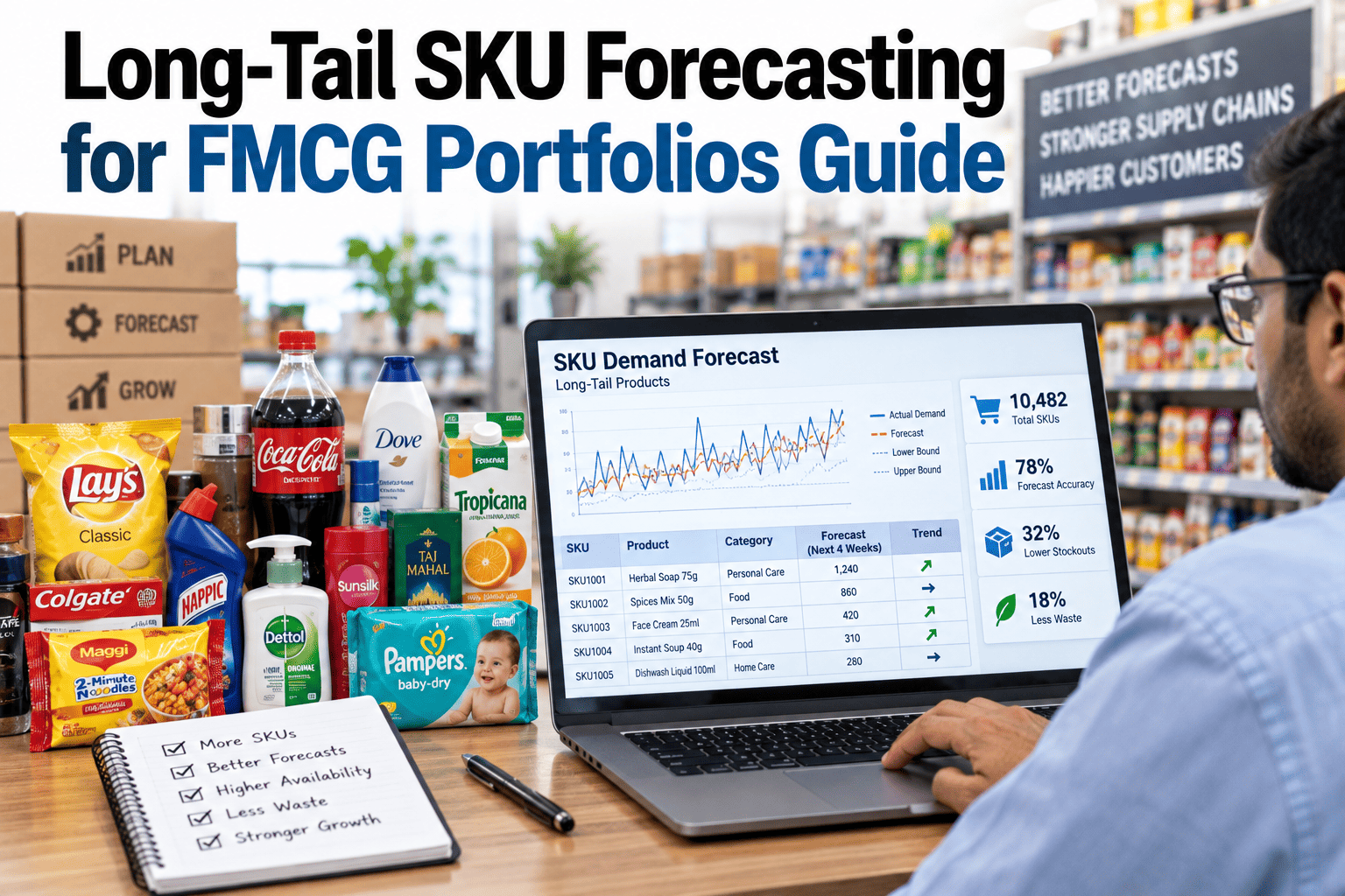
A typical FMCG portfolio has a small number of SKUs that drive most of the volume and a very long list of SKUs that sell sporadically — a few units one week, none for the next three, then a small burst. Standard forecasting methods built for smooth, continuous demand tend to fall apart on this long tail, either predicting demand that never materializes or missing it entirely when it does. Planners managing thousands of these low-volume SKUs can Book a Demo to see how iFactory handles intermittent demand at portfolio scale.
The Shape of a Typical FMCG Portfolio
Plot total sales volume against SKU count for almost any FMCG portfolio and the same shape appears every time — a short, steep head of high-volume SKUs, a broader torso of moderate sellers, and a long, flat tail of SKUs that individually contribute very little volume but collectively make up a large share of the total SKU count a planner has to manage. The tail is where standard forecasting approaches struggle most, because the demand pattern there isn't smoothly continuous — it's intermittent, arriving in sporadic bursts separated by stretches of zero sales.
Why Standard Forecasting Methods Fail on Intermittent Demand
Standard time series methods assume demand occurs continuously and smoothly, which makes them fundamentally mismatched to a SKU that sells three units, then nothing for five weeks, then two units. Applied to this kind of pattern, standard methods tend to either forecast a small constant trickle of demand every week — leading to chronic overstock during the zero-sales weeks — or overreact to each sporadic sale as if it signals a new trend, leading to a whipsaw of forecast revisions that erodes planner trust in the system entirely.
Intermittent demand modeling methods, most notably Croston's method and its variants, address this directly by separating the forecast into two distinct components: how often demand occurs at all, and how large a typical demand event is when it does occur. Forecasting these two components separately, rather than trying to smooth them into a single continuous prediction, produces a far more realistic picture of what a long-tail SKU's demand actually looks like.
Croston's Method and the TSB Variant
Croston's method forecasts intermittent demand by separately tracking the average size of a demand event and the average interval between events, combining the two into a forecast rather than trying to predict a single smoothed weekly number. It works well for many long-tail SKUs, but it has a known limitation on items with a genuine and lasting decline in demand, since it can be slow to recognize that a SKU's demand interval is stretching out permanently rather than fluctuating temporarily.
The TSB variant, short for Teunter-Syntetos-Babai, addresses this limitation by modeling the probability of demand occurring in a given period directly, rather than the interval between events, which makes it more responsive to items whose demand is genuinely declining toward obsolescence. Choosing between Croston and TSB, or blending both depending on a SKU's observed demand trajectory, is a meaningful accuracy lever that a one-size-fits-all forecasting approach misses entirely.
| Method | Best Fit | Known Limitation |
|---|---|---|
| Croston's method | Stable intermittent demand without a lasting trend | Slow to recognize genuine long-term decline |
| TSB variant | SKUs trending toward decline or obsolescence | Can be more sensitive to short-term noise on very stable items |
| Standard time series | Continuous, high-volume demand only | Consistently underperforms on sporadic, low-volume SKUs |
Hierarchical Reconciliation: Making Thousands of Forecasts Consistent
Forecasting thousands of individual long-tail SKUs independently creates a subtle but costly problem — the sum of all those individual SKU forecasts often doesn't match a more reliable aggregate forecast at the category or brand level, where volume is higher and the signal is cleaner. Hierarchical reconciliation resolves this by forecasting at multiple levels of the product hierarchy simultaneously and adjusting the individual SKU-level forecasts so they add up consistently to the more trustworthy aggregate number, borrowing strength from higher-volume levels to stabilize the noisier SKU-level detail.
This matters enormously for long-tail SKUs specifically, since an individual low-volume item's own history often isn't sufficient on its own to produce a stable forecast, but the category it belongs to almost always has a clear, well-behaved pattern that can inform a more sensible allocation down to the SKU level.
Frequently Asked Questions: Long-Tail SKU Forecasting for FMCG
How do we decide which SKUs qualify as long-tail versus torso in our own portfolio?
A practical starting point ranks SKUs by trailing volume and draws the boundary where sales frequency drops below a consistent weekly pattern — SKUs selling every week in meaningful quantity generally sit outside the long tail, while those with frequent zero-sales weeks fall inside it. The exact cutoff varies by category and portfolio size, so validating the boundary against actual forecast performance for SKUs near the threshold refines it over time. Teams can Book a Demo to review this segmentation for a specific portfolio.
Does hierarchical reconciliation require a perfectly clean product hierarchy to work?
A reasonably well-structured hierarchy improves reconciliation quality significantly, but the method can tolerate some inconsistency and still produce meaningfully better results than forecasting every SKU in isolation. That said, cleaning up major hierarchy gaps — SKUs miscategorized or missing a category assignment entirely — before implementation is worth the effort, since those gaps limit how much benefit reconciliation can provide.
How much history is needed before intermittent demand modeling produces reliable results?
Intermittent demand methods generally need less history than standard time series models to start producing usable results, since they're specifically designed for sparse data, but a minimum of several months covering multiple demand events is still preferable to build a stable estimate of both event size and frequency. Brand-new SKUs with almost no history typically rely on analog-product comparisons until enough of their own data accumulates.
Should long-tail SKUs get the same forecast review frequency as high-volume SKUs?
Reviewing thousands of long-tail SKUs individually every planning cycle isn't practical or necessary, so most mature planning processes review long-tail forecasts by exception — flagging only SKUs whose forecast changed significantly or whose actual sales deviated sharply from prediction — while reserving detailed manual review for the smaller set of high-volume SKUs where accuracy has the largest business impact.
Can long-tail SKUs be discontinued based on forecast output alone?
Forecast output showing consistently low or declining demand is a useful input to a discontinuation decision, but it shouldn't be the sole factor — some long-tail SKUs exist deliberately for strategic reasons like completing a product line or serving a specific customer segment, and a forecasting system has no visibility into that context. Combining forecast signal with commercial and strategic review produces better discontinuation decisions than automating them purely off predicted volume. Contact iFactory Support for guidance on structuring this combined review process.