Two culverts installed the same year, from the same material, in the same district can have completely different remaining lives — one exposed to heavier truck loading, one sitting in more corrosive soil, one inspected twice as often as the other. A fixed replacement schedule cannot see any of that difference; it treats both culverts as identical because they share an install date. Remaining useful life prediction replaces that guess with a running estimate built from condition history, sensor data, and environmental exposure for each individual asset. iFactory's RUL models turn scattered inspection and sensor records into a defensible, asset-by-asset forecast your capital plan can actually rely on — reach out to see it applied to your own portfolio.
PREDICTIVE ASSET MANAGEMENT — RUL
AI Infrastructure Remaining Useful Life Prediction Software
Predict remaining useful life for infrastructure assets using condition history, sensor data, environmental factors, and AI models trained on how your assets actually deteriorate — not on a generic replacement table.
15–25%
Typical extension in asset service life achieved through condition-based prediction
62%
Reduction in unplanned expenses reported when predictive approaches replace fixed schedules
8%
Capital expenditure savings from optimizing replacement timing instead of guessing early
$125B
National bridge maintenance backlog that better lifecycle forecasting is built to shrink
What Actually Feeds a Remaining Useful Life Model
A useful RUL estimate is never built from a single data source. It is a running synthesis of everything known about how an asset has aged so far, weighted by how strongly each factor actually correlates with the failure modes that matter for that asset class. The categories below are the inputs iFactory's models draw on, and each one sharpens the forecast in a different way.
Condition History
Every past inspection score, defect record, and repair event for the specific asset, establishing the actual decay trajectory rather than an assumed average curve.
Sensor & IoT Data
Vibration, strain, moisture, tilt, and corrosion-rate readings from installed sensors, where available, giving the model a continuous signal between inspection cycles.
Environmental Exposure
Climate zone, freeze-thaw cycles, salt exposure, soil chemistry, and flood history — the external stressors that accelerate or slow deterioration independent of asset age.
Load & Usage Intensity
Traffic volume, vehicle weight class, throughput, or operating hours — how hard the asset is actually being used relative to its original design assumptions.
Materials & Construction Record
Original material specification, construction method, and known batch or supplier issues that make certain cohorts of assets deteriorate faster than their peers.
Maintenance & Repair Records
What repairs were made, when, and how the asset's condition trend responded afterward — data that reveals whether past interventions actually extended service life.
Fixed Schedule vs RUL-Driven Replacement
Most infrastructure portfolios still plan capital replacement around a generic assumed lifespan by asset type, which forces a choice between replacing too early and wasting remaining service life, or replacing too late and risking failure. The comparison below shows why that choice is unnecessary once individual asset forecasting is available.
| Planning Dimension | Fixed Schedule Replacement | RUL-Driven Replacement |
|---|
| Basis for timing | Assumed average lifespan by asset type | Individual asset condition and decay trajectory |
| Early replacement waste | Common — healthy assets replaced on schedule | Minimized — assets used to their actual limit |
| Failure risk | Higher — some assets fail before their scheduled date | Lower — declining assets flagged before failure |
| Budget forecasting | Lump-sum estimates by cohort and year | Asset-level forecast with confidence bands |
| Data required | Install date and asset type only | Condition history, sensor data, environmental factors |
The Deterioration Curve — Four Stages the Model Tracks
Assets do not fail on a straight line. Deterioration typically holds nearly flat for years, then accelerates once a threshold is crossed, then accelerates again as one failure mode begins compounding another. iFactory's models track which stage an asset currently sits in and how quickly it is moving toward the next one, rather than reporting a single static age-based number.
STABLE
Condition holds flat with only minor, expected wear. Decay rate is slow and forecast confidence is high for a long remaining window.
EARLY DECLINE
First measurable defects appear. Decay rate begins to increase gradually, and the model narrows its remaining-life confidence band.
ACCELERATING
Multiple defect types compound each other. Decay rate increases sharply, and the remaining useful life estimate shortens with each new inspection.
END OF LIFE WINDOW
Asset approaches its minimum acceptable condition threshold. Replacement or major rehabilitation planning should already be underway by this stage.
Most agencies discover that a large share of their portfolio sits comfortably in the Stable or Early Decline stages at any given time, while a small, disproportionately expensive subset has quietly moved into the Accelerating or End of Life Window stages without anyone noticing on the standard inspection cycle. Surfacing that subset early, rather than waiting for the next scheduled walk-through to catch it, is where most of the financial value of remaining useful life forecasting actually shows up.
See a Remaining Useful Life Forecast Built From Your Own Asset Data
iFactory can run a sample forecast against a subset of your existing condition, sensor, or maintenance records so you can compare it directly against your current replacement schedule.
Asset Classes — How the Forecast Changes by Type
The factors that dominate a remaining-life forecast differ sharply by asset class, so the model weighting is never one-size-fits-all across a portfolio.
Roads & Pavement
Traffic loading and freeze-thaw cycles dominate the forecast, with surface condition trend as the primary leading indicator of remaining structural life.
Bridges & Structures
Element-level condition history and corrosion progression on structural steel and rebar carry the heaviest weight, refined further where sensor data exists.
Pipelines & Utilities
Soil chemistry, material type, and internal corrosion or lining condition drive most of the variance in remaining life across a buried utility network.
Buildings & Facilities
Envelope and roof condition trend combine with usage intensity and climate exposure to forecast remaining life on major building systems and components.
From Data Ingestion to a Confidence-Banded Forecast
A remaining useful life number without a confidence range invites false precision. iFactory's pipeline is built to produce both the estimate and the honest uncertainty around it, so capital planners can weigh the forecast appropriately against other budget priorities.
1
Data Ingestion
Condition records, sensor feeds, maintenance history, and environmental data are pulled together into a single asset-level timeline.
2
Decay Curve Fitting
The model fits the asset's actual observed decay pattern against similar assets' historical run-to-failure curves for the same class and conditions.
3
RUL Estimation
A remaining useful life value is calculated for the asset, expressed in time or condition-cycles remaining until the defined minimum threshold.
4
Confidence Banding
A confidence range is attached to the estimate based on data completeness and historical model accuracy for that asset class.
5
Capital Plan Integration
Forecasts feed directly into replacement prioritization and multi-year capital budgeting, updated automatically as new data arrives.
A Capital Planning Director on What the Forecast Changed
"
Our capital plan used to be built almost entirely on installation dates, which meant we were replacing some assets that had a decade of good service left in them while other assets that were genuinely struggling didn't get flagged until an inspection happened to catch them. Once we had a remaining-life estimate attached to each asset instead of just an age, the conversation with our finance committee changed completely. We could show them why a specific culvert needed to move up in the queue and why a specific bridge deck we'd planned to replace next year could safely wait three more years, and both of those decisions were backed by the same underlying data instead of two different people's gut instinct. The confidence bands mattered more than I expected going in — being able to say we were reasonably certain about some estimates and less certain about others, because the sensor coverage on the second group was thinner, gave the committee a level of honesty they said they hadn't seen in a capital request before.
— Capital Planning Director, Regional Public Works Agency · 18 Years Asset Lifecycle Management
What Changes in the First 90 Days
Building a reliable remaining useful life forecast does not require years of sensor history before it produces value. The milestones below reflect what pilot deployments typically achieve within a single quarter on an initial asset cohort.
Days 1–14
Historical data consolidated
Existing condition, maintenance, and sensor records for pilot assets are pulled together into a single structured timeline per asset.
Days 15–30
First forecasts generated
Initial remaining useful life estimates and confidence bands are produced for the pilot cohort and compared against current replacement schedules.
Days 31–60
Model refined against new data
New inspection and sensor data flowing in during the pilot sharpens the forecast and narrows confidence bands where coverage is strongest.
Days 61–90
Capital plan reprioritized
Forecasts feed a first pass at reprioritizing the replacement queue, identifying both accelerated and deferred candidates within the pilot set.
Common Pitfalls When Building an RUL Program
Organizations that see real value from remaining useful life forecasting tend to avoid a handful of predictable missteps in the early stages. The patterns below show up repeatedly and are worth planning around before the first forecast gets built into a budget decision.
Treating the Estimate as Exact
A remaining useful life number without its confidence band gets treated as fact by budget reviewers, which sets up disappointment when actual timelines shift. Always present the range, not just the point estimate.
Ignoring Data Quality Gaps
Feeding the model inconsistent inspection scoring across different inspectors and years without normalizing for that variance produces a forecast that inherits all the original inconsistency.
Modeling Every Asset Class the Same Way
A single generic deterioration curve applied across pavement, bridges, pipelines, and buildings ignores how differently each material and failure mode actually behaves under stress.
Never Updating the Forecast
A remaining useful life estimate generated once and left unchanged for years is no better than a fixed schedule — the value comes from refreshing it as new condition and sensor data arrives.
Skipping Engineering Sign-Off on High-Stakes Assets
For critical, high-consequence assets, the model's forecast should inform an engineering review rather than automatically trigger a final capital decision on its own.
Building the Business Case Around One Asset
A single success story is not a program. The real financial case for RUL forecasting shows up at the portfolio level, once dozens or hundreds of assets are being forecast and reprioritized together.
Is Your Portfolio Ready for Remaining Useful Life Forecasting?
Before committing to a full rollout, it helps to honestly assess where your organization stands on the fundamentals that determine whether an RUL program will produce trustworthy forecasts quickly or stall out during onboarding.
You Have Historical Condition Records
Even a partial inspection history per asset gives the model something real to fit a decay curve against, rather than starting from a purely theoretical assumption.
You Can Identify Your Highest-Consequence Assets
A pilot delivers the most value when it starts on the assets where an early or late replacement decision carries the biggest financial or safety consequence.
Your Capital Planning Process Can Absorb New Inputs
A forecast only changes outcomes if the capital budgeting process has a defined place for it to plug into — confirm that workflow exists before the first forecast is generated.
Your Engineers Are Ready to Review Early Forecasts
Early involvement from the engineers who will ultimately defend the forecast to a finance committee builds the trust that determines whether the program sticks past the pilot phase.
Frequently Asked Questions
How much historical data do we need before RUL predictions become useful?
Useful forecasts can begin with as little as a handful of past inspection records per asset, since the model also draws on run-to-failure patterns from similar assets across your portfolio and, where relevant, industry benchmark data for the same material and asset class. Forecast confidence naturally improves as more of your own condition history and sensor data accumulate, but a thin data history is treated as a wider confidence band rather than a reason to withhold an estimate entirely. Sparse-data assets are always flagged as lower confidence so planners know exactly how much weight to give each number.
Do we need IoT sensors installed for this to work, or can it run on inspection data alone?
Sensor data sharpens the forecast and narrows confidence bands, particularly between inspection cycles, but it is not a prerequisite for a first useful estimate. Many organizations start RUL forecasting using only existing condition inspection records, maintenance history, and environmental data, then add targeted sensor coverage later on the specific assets where a narrower forecast window would meaningfully change a capital decision.
Our team can help identify which assets in your portfolio would benefit most from added sensor coverage first.
How does the model account for assets that received repairs partway through their life?
Repair and maintenance events are logged as part of each asset's timeline and treated as inflection points in the decay curve rather than being ignored or averaged away. The model learns how much a given repair type historically extends service life for that asset class, so a well-executed rehabilitation genuinely resets part of the forecast, while a repair that only masked a symptom without addressing the underlying cause is reflected in a shorter subsequent life estimate once new condition data confirms the pattern.
Can remaining useful life forecasts be trusted for actual budget submissions?
Forecasts are delivered with explicit confidence bands precisely so they can support real budget submissions without overstating certainty. Rather than presenting a single point estimate as fact, the output shows a likely range and the data completeness behind it, which finance committees and capital review boards generally find more credible than a bare age-based assumption. Many organizations use the forecast as the primary evidence for prioritization while still applying standard engineering review before finalizing a specific replacement date.
What does it cost to pilot RUL prediction across an initial asset cohort?
Pilot cost scales with the number of assets, the volume of historical data to be consolidated, and whether any supplemental sensor deployment is included in the initial scope. Because most pilots begin using data your organization already holds, first-phase costs are typically limited to data integration and modeling work rather than new hardware. The clearest way to see a realistic number against your own portfolio size is to
book a demo and walk through a scoped pilot with our team.
Stop Replacing Assets by Age — Replace Them by Actual Remaining Life
A fixed replacement schedule treats every asset the same regardless of how it has actually aged. iFactory's remaining useful life models turn condition history, sensor data, and environmental factors into a defensible, asset-by-asset forecast — so capital dollars go where the risk actually is, not where the calendar happens to point.