Traditional MRP was built on an assumption that stopped being true decades ago: that demand is forecastable enough, and lead times stable enough, for a single planned order to reliably arrive when the system says it will. Every plant manager who has watched a well-calculated MRP plan fall apart the moment one supplier ships late or one forecast misses knows the real cost of that assumption — nervousness. Small changes upstream cascade into constant re-planning, expedites, and a planning team spending more time firefighting than planning. Demand-Driven MRP replaces that fragile chain with strategically placed buffers that absorb variability instead of amplifying it, and AI is what makes those buffers accurate enough to trust. This guide covers how DDMRP works, where AI improves on the standard methodology, which SKUs typically see the biggest return, and how a demo can show AI-tuned buffers running against your own SKU data.
Why Traditional MRP Breaks Down Under Real-World Variability
Conventional MRP works by exploding a forecast through the bill of materials and generating planned orders based on that forecast, lead times, and current inventory. The math is precise, but it's precise about the wrong thing: it assumes the forecast is accurate and the lead time is stable, and it recalculates the entire plan every time either assumption is violated, which in practice is almost constantly. A late supplier shipment, a demand spike on one SKU, or a longer-than-expected changeover ripples through every downstream planned order, triggering a wave of re-planning that planners refer to, accurately, as nervousness — the plan changes so often that nobody fully trusts what it's telling them on any given day.
DDMRP addresses this problem at a structural level rather than simply trying to forecast demand more accurately than before. Instead of chaining every order to a forecast, it positions strategic decoupling points — usually key components or finished goods with high variability or long lead times — and protects them with a buffer sized to absorb normal variability without triggering a re-plan every time reality deviates slightly from the forecast. Demand signals still flow through the system, but the buffer acts as a shock absorber, decoupling the volatility of actual demand from the stability the rest of the plan needs to function.
The Three Buffer Zones That Drive Every DDMRP Decision
Every buffered SKU in a DDMRP system is divided into three color-coded zones, and the position of on-hand-plus-on-order inventory within those zones drives every replenishment decision, replacing the reorder-point logic of traditional MRP with a visual, immediately actionable signal.
A planner reading a DDMRP dashboard doesn't need to interpret a complex MRP exception report — the zone itself is the signal. Deep into red means order now. Comfortably in yellow or green means no action is required. This visual simplicity is a large part of why DDMRP reduces planner workload, but it only works well if the buffer boundaries themselves are sized correctly, which is exactly the part traditional DDMRP implementations tend to get wrong, leaving planners with a clean-looking dashboard built on inaccurate zone math underneath it.
Where Standard DDMRP Buffer Sizing Falls Short
The official DDMRP methodology sizes buffers using average daily usage, lead time, and a variability factor, typically set manually by category and reviewed on a periodic cycle. That approach is a significant improvement over static reorder points, but the manual variability factor is still a blunt instrument — it's usually set once per SKU category rather than tuned to the actual demand pattern of each individual SKU, which means a genuinely erratic item and a mildly seasonal item in the same category can end up with buffers sized almost identically, even though their true variability is nothing alike.
How AI Tunes DDMRP Buffers Dynamically
AI doesn't replace the DDMRP methodology — it replaces the manual, periodic buffer-sizing step with a model that continuously learns each SKU's actual demand and lead time pattern and adjusts the buffer zones accordingly. Instead of one variability factor applied to a whole category, each SKU gets a buffer shaped by its own statistical behavior, updated as new data arrives rather than waiting for the next scheduled review.
DDMRP Buffer Zones at a Glance
| Zone | Purpose | Typical Planner Action |
|---|---|---|
| Red | Protects against demand and supply variability | Expedite or urgently trigger replenishment |
| Yellow | Covers average demand across average lead time | Normal replenishment order, no urgency |
| Green | Governs order frequency and minimum order size | No action needed; buffer is healthy |
Common Gaps in DDMRP Implementations
Where DDMRP Delivers the Clearest Return
DDMRP isn't equally valuable in every planning environment. Its biggest impact shows up where traditional forecast-driven MRP struggles most: long or variable supplier lead times, demand patterns that are genuinely erratic rather than smoothly seasonal, and bill-of-material structures where a shared component feeds multiple finished goods, making any single forecast error ripple across an entire product family. A plant manager trying to decide whether a DDMRP pilot is worth the effort should look first at which SKUs are currently generating the most planner override activity — those are usually the items where a forecast-driven approach is most clearly mismatched to how demand actually behaves.
Building the case for a plant floor or supply chain leadership team is usually most effective when framed around the two costs that DDMRP most directly and consistently reduces, once buffers are sized correctly for each individual SKU rather than for a broad category average: carrying cost on excess inventory sitting against low-variability SKUs, and the expedite and premium freight cost triggered by stockouts on high-variability ones. Because AI-tuned buffers are sized correctly in both directions rather than uniformly wide or uniformly tight, plants typically see a reduction in both categories of cost simultaneously, which is a meaningfully easier number to defend to a finance stakeholder than a project that trades one metric for the other.
Getting Started Without Rebuilding Your Planning System
A plant manager evaluating AI-augmented DDMRP doesn't need to rip out an existing MRP or ERP system to get started. The buffer-sizing logic sits as a layer on top of existing planning data — historical demand, lead time actuals, and current on-hand and on-order positions — and produces recommended zone boundaries that planners can review before they go live, rather than requiring a full re-platform. Most plants start with a pilot group of ten to twenty high-variability or high-value SKUs, validate that the recommended buffers perform better than the current sizing over a full quarter, and then expand coverage once the approach has proven out against real service and inventory results rather than a theoretical model.
The SKUs that benefit most from this kind of pilot are usually the ones causing the most planner frustration already — items with a history of both stockouts and excess inventory at different points in the year, which is a strong signal that the current buffer sizing is wrong in both directions rather than simply too conservative or too aggressive. Starting there gives the clearest, fastest proof point, because the contrast between the old sizing and the new one tends to be largest exactly where the pain has been most visible to the planning team.
It's also worth setting expectations correctly before the pilot begins: DDMRP is not a one-time project that gets configured once and left alone, even with AI handling the ongoing sizing. Supplier performance shifts, demand patterns evolve, and new SKUs enter the portfolio constantly, which is exactly why continuous recalculation matters more than a more sophisticated one-time calculation would. A plant manager who treats the pilot as proof that the approach works, rather than as a finished implementation, sets the program up to keep delivering value well past the initial quarter of validation, since the same continuous recalculation that made the pilot successful is what keeps every subsequent quarter's buffers accurate as conditions keep changing.