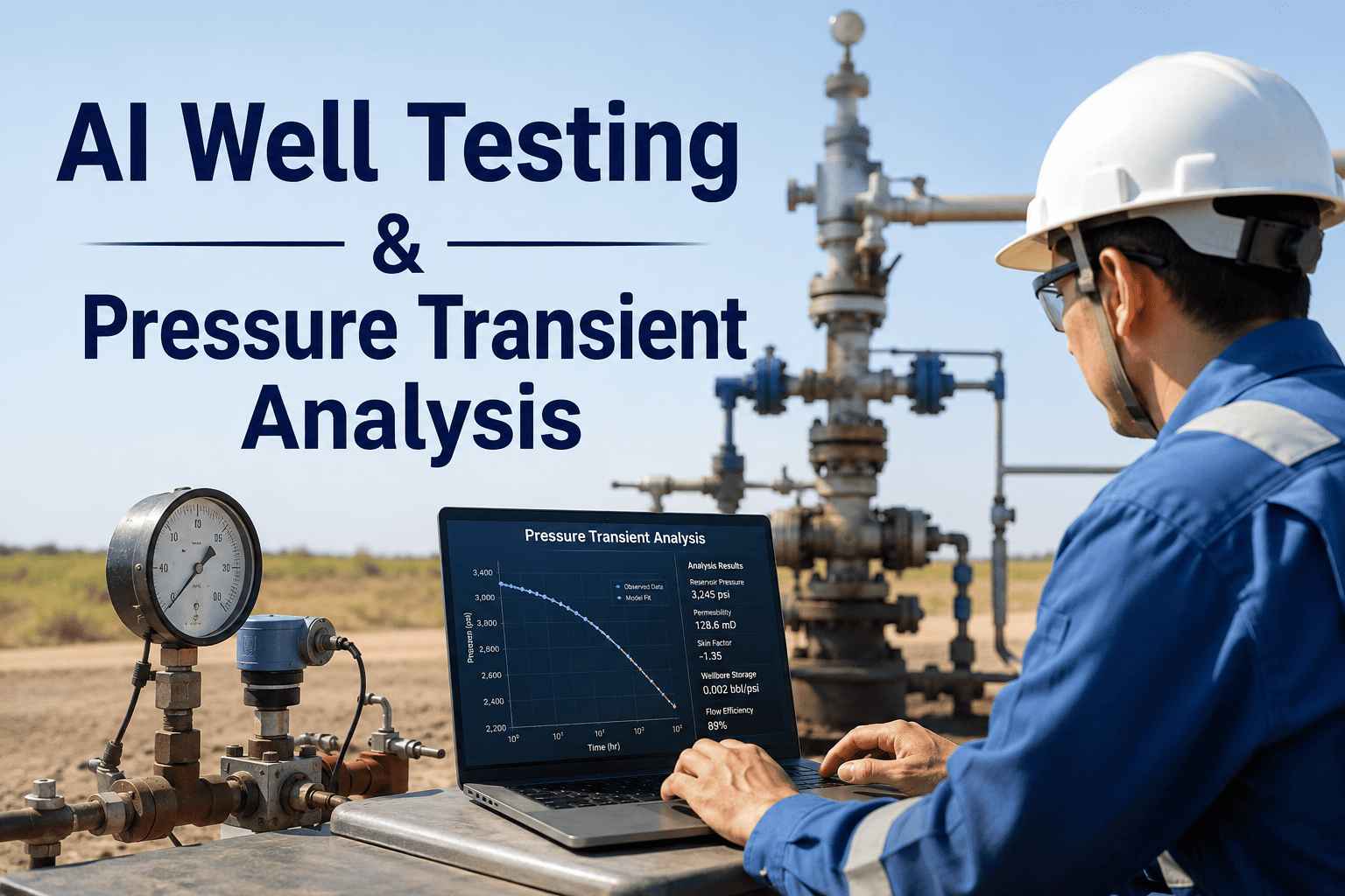
Pressure transient analysis has depended on expert interpreters staring at derivative plots for decades — identifying flow regimes by eye, matching straight-line segments, and arguing over whether a half-slope is bilinear flow or boundary effects. A single well test can take days to interpret manually, and two equally qualified petroleum engineers will often produce different reservoir models from the same data. AI changes this by turning pressure and rate data into consistent, repeatable interpretations in minutes instead of days. This article breaks down exactly what AI-driven PTA automates, where it outperforms manual methods, and how upstream teams are deploying it. Walk through your own well test data when you book a demo.
AI WELL TESTING · PRESSURE TRANSIENT ANALYSIS · FLOW REGIME · RESERVOIR CHARACTERIZATION
From days of manual derivative matching to minutes of automated reservoir interpretation
AI-driven pressure transient analysis identifies flow regimes, estimates reservoir parameters, and detects boundaries with consistency that no manual interpreter can match at scale.
Pressure Data
Gauge readings, rate history, time stamps
Regime ID
Flow regime classification per time region
Parameters
Permeability, skin, pressure, boundaries
Reservoir Model
Calibrated description for simulation
95%+
Flow regime classification accuracy on validated test sets.
Under 5 min
Full PTA interpretation from raw data to parameter report.
Zero Variance
Same data, same model, every time — no interpreter bias.
6+ Regimes
Radial, linear, bilinear, spherical, storage, boundary-dominated.
What pressure transient analysis actually measures
PTA extracts reservoir properties from the way pressure responds when a well's rate changes. Every transient carries information about the formation near the wellbore, the connected drainage volume, and the boundaries that limit flow. AI reads all three layers simultaneously instead of analyzing them in sequence.
01
Reservoir Permeability
How easily fluid moves through the rock matrix. Estimated from the pressure derivative during radial flow, this single parameter controls well productivity, reserve estimates, and completion design decisions.
02
Skin Factor
Quantifies near-wellbore damage from drilling fluid invasion or stimulation improvement from fracturing. A positive skin means reduced flow; a negative skin means the completion is outperforming the formation.
03
Initial Reservoir Pressure
The static pressure the reservoir held before production began. Critical for material balance calculations, drive mechanism identification, and determining whether pressure maintenance is needed.
04
Boundary Conditions
Sealing faults, channel boundaries, constant-pressure aquifers, and pinchouts that appear as derivative deviations at late time. These define the drainage geometry that simulation models must honor.
Five bottlenecks that make manual PTA unreliable at scale
Manual interpretation works on a single well test with clean data and an experienced engineer. It breaks when you need to interpret hundreds of tests per year across multiple basins with varying data quality. These are the five failure points that AI eliminates.
01
Derivative Smoothing Bias
The Bourdet derivative requires a smoothing window, and the window size changes the shape of the derivative curve. Two interpreters using different windows will identify different flow regimes from identical data — and neither is objectively wrong.
02
Subjective Regime Identification
Recognizing a half-slope as linear flow versus a quarter-slope as bilinear flow depends on visual judgment. On noisy data from low-permeability formations, the slope is ambiguous and interpreters disagree on which regime is present.
03
Non-Unique Straight-Line Fits
Horner, MDH, and pressure-pressure plots each require selecting a straight-line segment. The segment you choose determines the permeability and skin you calculate. Multiple valid segments often exist, leading to multiple valid but conflicting answers.
04
Manual Type Curve Matching
Overlaying field data on dimensionless type curves is iterative and non-unique. Slight shifts in the match point change permeability, skin, and storage coefficient simultaneously, and the interpreter must judge which combination is geologically plausible.
05
Cross-Well Inconsistency
When different engineers interpret tests from the same field using different methods, the resulting reservoir models are inconsistent. Simulation teams then spend weeks reconciling conflicting PTA results before they can build a coherent field model.
AI-driven PTA versus manual interpretation
Every step in the PTA workflow has a manual method and an AI method. The table below shows where AI delivers a clear advantage and where manual methods still hold value — so you know exactly what to automate and what to keep human-led.
| PTA Task | Manual Method | AI Method | Recommendation |
| Derivative calculation |
Bourdet with fixed window |
Adaptive multi-scale smoothing |
AI-driven |
| Flow regime identification |
Visual slope recognition |
Classification on derivative features |
AI-driven |
| Permeability estimation |
Straight-line analysis |
Regression on regime-matched model |
AI-driven |
| Skin factor calculation |
Type curve match point |
Joint inversion with permeability |
AI-driven |
| Boundary detection |
Late-time derivative deviation |
Probabilistic boundary mapping |
AI-driven |
| Geological plausibility check |
Engineer judgment |
No direct substitute |
Human-led |
| Test design and planning |
Experience-based duration estimate |
Simulated test with noise model |
AI-assisted |
| Regulatory reporting |
Manual report assembly |
Auto-generated with evidence |
AI-driven |
Six flow regimes the AI classification engine detects
Each flow regime produces a characteristic slope on the pressure derivative plot. The AI model is trained to identify these slopes even when noise, gauge drift, and rate fluctuations obscure the ideal signature. Here is what it looks for.
1.0 SLOPE
Wellbore Storage
Early-time unit slope on the derivative indicates fluid compressibility in the wellbore dominates the pressure response. The AI estimates storage coefficient from the duration and magnitude of this regime.
0.0 SLOPE
Radial Flow
Horizontal derivative plateau is the most important regime — it yields permeability and skin. The AI isolates the plateau even when storage transition distorts the early portion of the radial period.
0.5 SLOPE
Linear Flow
Half-slope indicates flow through a narrow channel, along a hydraulic fracture, or between parallel faults. The AI distinguishes linear flow from bilinear by analyzing both the derivative and the pressure integral simultaneously.
0.25 SLOPE
Bilinear Flow
Quarter-slope is specific to finite-conductivity hydraulic fractures where pressure drop occurs in both the fracture and the formation. The AI detects this regime and estimates fracture conductivity directly.
-0.5 SLOPE
Spherical Flow
Negative half-slope appears in partially penetrating wells or thick formations with limited completion intervals. Rare but diagnostic — the AI flags it when it appears rather than misclassifying it as noise.
RISING
Boundary-Dominated
Derivative rising above the radial flow plateau signals that the pressure transient has reached a reservoir boundary. The AI maps the shape of the rise to identify fault geometry, channel width, or constant-pressure support.
Reservoir parameters the model estimates from each test
Every completed PTA interpretation produces a parameter set that feeds directly into reservoir models, completion evaluations, and reserve estimates. The AI extracts all of them in a single pass rather than requiring separate analyses for each parameter.
kh
250 mD·ft
Permeability-thickness product from radial flow derivative plateau. Foundation for productivity index and inflow performance.
S
-2.1
Skin factor indicating stimulated wellbore. Negative values confirm effective fracture or acid treatment.
Pi
4,850 psi
Initial reservoir pressure from Horner extrapolation or model-based estimation. Key input for material balance.
re
750 ft
Drainage radius estimated from the time boundary effects first appear on the derivative.
C
0.02 bbl/psi
Wellbore storage coefficient from early-time unit slope. Determines how long the storage regime masks radial flow.
Fcd
12.4
Dimensionless fracture conductivity for hydraulically fractured wells. Estimated when bilinear flow is detected.
See AI pressure transient analysis running against your well test data
iFactory trains the PTA model on your formation types, gauge configurations, and test designs — so every interpretation is calibrated to your reservoir instead of a generic model.
Buildup versus drawdown: AI handles both without separate workflows
Buildup and drawdown tests produce different pressure signatures but carry the same reservoir information. Manual interpretation often treats them as separate problems with different analysis methods. AI unifies them under a single model that accounts for the superposition effects each test type introduces.
BUILDUP TEST
Well shut in after production
Pressure recovers toward reservoir pressure as the disturbance from production dissipates. The derivative plot shows flow regimes in reverse order — boundary effects first, then radial, then storage. AI applies superposition in time to deconvolve the production history and extract the same parameters a drawdown test would reveal.
Rate superposition handled automatically
Cleaner signal — well is not flowing
Reverse regime sequence recognized by model
Horner time conversion built into inference
DRAWDOWN TEST
Well flowing at constant rate from shut-in
Pressure declines as the drainage radius expands outward. The derivative shows regimes in forward order — storage, radial, then boundaries. Surface rate fluctuations and multiphase flow effects introduce noise that AI filtering removes without destroying the transient signal.
Real-time rate correction during flow
Multiphase flow noise filtered adaptively
Forward regime sequence is standard classification
Continuous interpretation during extended tests
Boundary detection: what the AI sees at late time
When the pressure transient reaches the edge of the reservoir, the derivative deviates from the radial flow plateau. The shape of that deviation encodes the boundary geometry. Manual interpreters recognize a handful of common patterns. The AI maps the full probability distribution across boundary models and quantifies uncertainty for each.
SINGLE FAULT
Sealing Fault
Derivative doubles and stabilizes at a new plateau. The AI measures the distance to the fault from the time of the deviation and the permeability already estimated from radial flow.
CHANNEL
Parallel Faults
Derivative shows linear flow between two parallel boundaries before ultimately rising. The AI distinguishes this from a single fracture by analyzing the duration of the half-slope segment.
CLOSED
Rectangular Drainage
Derivative rises steeply as all boundaries are felt simultaneously. The AI fits the rising segment to rectangular models and estimates the drainage area dimensions from the timing of successive derivative breaks.
AQUIFER
Constant Pressure Support
Derivative drops below the radial plateau as pressure support from an aquifer or injection well stabilizes reservoir pressure. The AI identifies this from the downward trend and estimates the strength of pressure support.
INFINITE
No Boundary Detected
Derivative remains at the radial flow plateau through the entire test duration. The AI reports a minimum drainage radius based on the radius of investigation at the end of the test and flags whether the test was long enough to see boundaries.
Frequently asked questions
What well test data formats does the AI system accept?
The system accepts standard well test data formats including CSV pressure-time-rate arrays, Eclipse output files, Saphir-native formats, and direct OPC-UA connections to SCADA systems for real-time data ingestion. During deployment, iFactory maps your existing data pipelines to the ingestion layer so no manual data reformatting is needed. Both surface and downhole gauge data are supported, including dual-gauge configurations for gradient analysis.
Book a demo to test your data format against the ingestion pipeline.
How does AI handle noisy pressure data from low-rate wells?
Low-rate wells produce small pressure changes that are often buried in gauge noise, tidal effects, and thermal drift. The AI preprocessing layer applies adaptive denoising that preserves true transient response while removing gauge artifacts, something fixed-bandwidth filters cannot do because they discard the same frequency content that carries reservoir signal. The model then performs regime identification on the cleaned derivative rather than the raw data, which dramatically improves confidence on marginal tests.
Contact our support team for a noise assessment on your low-rate well data.
Can AI PTA replace reservoir simulation entirely?
No, and it should not try to. AI-driven pressure transient analysis is a diagnostic tool that estimates near-wellbore and drainage-area parameters from transient pressure and rate data. Reservoir simulation is a predictive tool that models fluid flow over time under production scenarios. The two are complementary: AI PTA provides the initial reservoir description including permeability distribution, skin, boundaries, and pressure that feeds into the simulation model as calibration points.
Book a demo to see how AI PTA output integrates with your simulation workflow.
What happens when the AI encounters a flow regime not in its training set?
The model assigns a low confidence score to regime classifications that do not closely match any trained pattern and flags the test for expert review rather than forcing an incorrect label. This is fundamentally different from rule-based systems that either match a template or return nothing. The AI provides a probability distribution across all known regimes and highlights which time regions are ambiguous. The flagged interpretations are fed back into the training set so the model improves with every unusual well test it encounters.
Contact our support team to understand the confidence threshold workflow.
How long does it take to deploy AI PTA on an active drilling program?
A typical deployment takes eight to fourteen weeks depending on the number of well types, data quality, and integration requirements with existing reservoir management software. The first phase covers data audit and cleaning, the second phase trains and validates models against your historical well tests, and the final phase connects to real-time data feeds and deploys the inference engine on-premise. Shadow-mode validation runs alongside your current interpretation workflow until the AI matches or exceeds expert accuracy on your specific formations.
Book a demo to scope a deployment timeline for your drilling program.
Turn well test interpretation from a bottleneck into a continuous automated workflow
iFactory delivers on-premise AI inference, adaptive derivative analysis, flow regime classification, and audit-ready parameter reports as a single stack. Book a demo and run the model against your next buildup test.