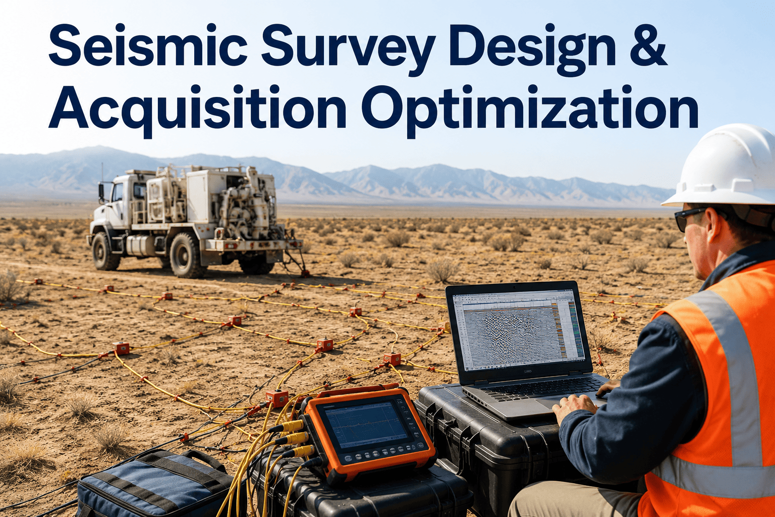
Every seismic survey represents a multi-million-dollar investment made before a single trace is processed, and the quality of that investment is locked in the moment the acquisition geometry is finalized. Source and receiver spacing, fold coverage, offset distribution, and azimuth range are all determined during survey planning — and once the crew mobilizes, none of them can be changed without starting over. Conventional survey design relies on rule-of-thumb parameters, simplified ray tracing, and spreadsheet-based cost estimates that optimize each parameter in isolation rather than evaluating the geometry as an integrated system. AI-driven survey simulation evaluates thousands of geometry configurations in hours, predicting the imaging impact of every parameter tradeoff and identifying the design that delivers maximum subsurface quality per dollar spent before the first shot is fired. Book a demo to see how iFactory simulates and optimizes your next seismic acquisition before you commit budget to the field.
SEISMIC DATA ANALYTICS · ACQUISITION PLANNING · OIL & GAS AI
Seismic Survey Design and Acquisition Optimization — Maximize Image Quality Per Dollar Before the First Shot
iFactory evaluates thousands of source-receiver geometries against your geological targets, predicting fold coverage, offset distribution, and azimuth sampling for each configuration — then ranks every design by imaging quality per acquisition dollar so your team chooses the right geometry with full confidence.
10,000+
Geometry Configurations Evaluated Per Survey
15-30%
Acquisition Cost Reduction Without Image Degradation
Hours
Full Survey Simulation Turnaround vs Weeks Manually
THE HIDDEN COST
How Suboptimal Geometry Degrades Your Final Seismic Image
The bars below represent the relative impact that each acquisition design parameter has on final image quality when it is underspecified or poorly distributed. These are not theoretical concerns — they are the specific failure modes that show up as migration artifacts, velocity ambiguity, and unresolved thin beds in the processed volume, and they cannot be fixed by processing after acquisition is complete.
Source-Receiver Spacing
Critical
Controls spatial sampling and aliasing. Undersampled spacing creates spatial aliasing that produces migration smiles and false events that no processing step can remove after acquisition.
Maximum and Minimum Offset
Critical
Maximum offset determines velocity resolution and deep reflector illumination. Minimum offset controls near-surface visibility and shallow reflector fidelity. Both must be specified together.
Fold Coverage Uniformity
High
Uneven fold creates amplitude variations that mimic geological features. Noise levels in low-fold bins can be 3-5 times higher than in adjacent high-fold bins, corrupting attribute analysis.
Azimuth Distribution
High
Narrow azimuth acquisition biases the velocity field and reduces the ability to resolve azimuthal anisotropy, leading to mispositioned faults and incorrect fracture orientation estimates.
Record Length and Sample Rate
Moderate
Truncated record lengths clip deep reflections and limit velocity analysis at depth. Excessively coarse sampling attenuates high frequencies and reduces vertical resolution of thin target intervals.
Source Effort and Sweep Parameters
Moderate
Insufficient source effort degrades signal-to-noise ratio below the threshold needed for coherent reflection imaging, particularly in noisy land environments or deep-water marine settings.
DESIGN PARAMETERS
Six Acquisition Decisions That Lock In Your Subsurface Image Before Acquisition Begins
Each parameter below is set during survey planning and cannot be modified once recording starts. The AI optimization engine evaluates the interaction between all six simultaneously — because changing source spacing without recomputing its effect on fold, offset, and azimuth distribution produces a design that looks efficient on paper but fails in practice.
Source Point Spacing
Determines the number of shot points per unit area and directly controls the CMP fold. Reducing source spacing increases fold and improves noise suppression but proportionally increases acquisition time and cost. AI evaluates the marginal imaging gain per additional source point to find the spacing where cost increases faster than quality improvement.
Receiver Line and Station Spacing
Controls cross-line spatial sampling and the maximum unaliased frequency in the cross-line direction. Receiver spacing also determines the minimum offset distribution within each CMP bin. AI models the full spatial wavefield to identify the coarsest receiver spacing that still prevents aliasing at your target frequency and dip.
Maximum Offset to Target Depth Ratio
Governs the angular illumination of subsurface reflectors and the resolution of velocity analysis. Longer offsets improve velocity resolution but introduce NMO stretch that degrades high-frequency content at far offsets. AI computes the stretch-free offset limit for your target depth and frequency band and optimizes the offset distribution around it.
Fold Coverage and Bin Size
Fold determines random noise reduction and the statistical reliability of amplitude measurements. Bin size sets the horizontal resolution of the final migrated image. AI simulates fold maps for each candidate geometry and flags bins that fall below your minimum fold threshold before acquisition, not after.
Azimuth Range and Distribution
Full-azimuth acquisition provides uniform illumination of complex structures and enables azimuthal anisotropy analysis. Narrow-azimuth designs are cheaper but create direction-dependent imaging artifacts. AI quantifies the azimuthal illumination gap for each geometry and predicts where narrow-azimuth designs will produce shadow zones at your target.
Record Length and Temporal Sampling
Record length must capture the deepest reflection of interest plus moveout at maximum offset. Sample rate must satisfy the Nyquist criterion for the highest frequency your source and target can support. AI calculates the minimum record length from your target depth and velocity model and validates the sample rate against your desired vertical resolution.
GEOMETRY COMPARISON
Acquisition Environment Determines Which Design Parameters Matter Most
Land, marine streamer, and ocean-bottom node surveys operate under fundamentally different constraints. The table below maps each environment to its critical design parameters, typical fold ranges, and the cost driver that AI optimization targets most effectively. Understanding these differences is essential because applying marine design rules to a land survey — or vice versa — is one of the most common sources of suboptimal acquisition geometry.
| Parameter |
Land Vibroseis |
Marine Streamer |
Ocean Bottom Nodes |
| Source Type |
Controlled sweep, multiple vibrators |
Air gun arrays, tuned to depth |
Air gun or source vessel |
| Receiver |
Geophones, cable or wireless nodes |
Hydrophone groups on streamers |
4C nodes on seabed |
| Typical Fold Range |
30-120 fold common |
40-300 fold typical |
Variable, often 200-1000+ |
| Offset Range |
Limited by permit boundaries |
Set by streamer length |
Set by source-receiver geometry |
| Azimuth Coverage |
Full azimuth typical |
Narrow, sail-line direction |
Full azimuth achievable |
| Primary Cost Driver |
Source point count and move-up time |
Streamer count and vessel days |
Node deployment and recovery time |
| AI Optimization Target |
Source line spacing and sweep efficiency |
Streamer spacing and sail line pattern |
Node density and shot patch design |
Your Survey Budget Is Finite — AI Finds the Geometry That Spends It on the Parameters That Actually Improve Your Image
iFactory simulates your acquisition geometry against your geological target before mobilization, showing your team exactly which design changes improve imaging and which ones just add cost.
AI SIMULATION PIPELINE
Four Stages from Geological Objective to Optimized Acquisition Geometry
The pipeline below represents the complete AI survey design workflow from initial objective definition through to a finalized, cost-optimized geometry ready for bid specification. Each stage produces a deliverable that your acquisition team can review and approve independently.
01
Geological Objective Definition
Target depth, minimum horizon thickness, required vertical resolution, structural dip range, and known velocity complexity are defined as quantitative constraints. These constraints become the evaluation criteria that every candidate geometry is tested against — not subjective descriptors but measurable imaging specifications.
02
Parameter Space Exploration
The AI engine generates thousands of candidate geometries by systematically varying source spacing, receiver spacing, line intervals, and recording parameters within the physical and logistical constraints of the survey area. Each geometry is a complete, self-consistent design — not a single parameter tweak in isolation.
03
Full-Wavefield Simulation and Scoring
Each candidate geometry is evaluated through forward wavefield modeling that predicts fold maps, offset histograms, azimuth rose diagrams, and spatial frequency response at the target depth. A composite imaging score is computed for every geometry by weighting each metric against the geological objectives defined in stage one.
04
Cost-Weighted Optimization
Acquisition cost is estimated for each geometry based on source point count, receiver requirements, recording time, and logistical constraints. Geometries are ranked by imaging quality per dollar, and the optimal design is identified as the point where additional spending yields diminishing imaging returns — not the cheapest design, but the most efficient one.
QUALITY PILLARS
Fold, Offset, and Azimuth — The Three Metrics That Predict Whether Your Design Will Image the Target
These three quantities are the fundamental output of any survey design analysis. They are also the three metrics that AI optimization evaluates simultaneously — because optimizing fold without checking offset distribution, or optimizing offset without checking azimuth, consistently produces geometries that score well on one metric and fail on the others.
Fold
Fold Coverage Uniformity
AI generates a fold map for every candidate geometry, computing not just the average fold but the standard deviation, the minimum fold in any bin, and the percentage of bins below your specified threshold. A design with high average fold but large low-fold holes will score lower than a design with slightly lower average fold but uniform coverage across the entire survey area.
Offset
Offset Distribution per Bin
For each CMP bin, the AI computes the full offset histogram and evaluates whether the distribution provides sufficient near-offset coverage for shallow targets, sufficient far-offset coverage for velocity resolution at depth, and uniform sampling across the full offset range. Bins with gaps in the offset histogram produce velocity ambiguity that cannot be resolved by processing.
Azim
Azimuth Sampling and Illumination
The AI generates azimuth rose diagrams for each bin and quantifies the angular illumination gap — the largest azimuth sector with no ray coverage. For complex structures with steep dips or azimuthal anisotropy, the optimization engine penalizes geometries with illumination gaps larger than a user-specified threshold, ensuring that the final design provides the azimuthal coverage your processing requires.
BEFORE AND AFTER AI
What Changes When You Replace Spreadsheet-Based Design with AI Simulation
The comparison below is not hypothetical — it reflects the consistent pattern of results that acquisition teams report when they move from manual, parameter-by-parameter design to AI-driven simultaneous optimization. The left column describes the workflow most teams use today. The right column describes what the same team does with the AI platform.
Traditional Spreadsheet-Based Design
Geometry Iterations Tested
5-15 manual configurations
Parameter Optimization Method
One parameter at a time, all others fixed
Fold and Offset Analysis
Calculated for final design only
Cost Estimation Timing
After geometry is finalized
Design Turnaround
2-6 weeks for a 3D survey
Confidence in Final Design
Based on limited parameter sweeps
AI-Optimized Survey Simulation
Geometry Iterations Tested
10,000+ automated configurations
Parameter Optimization Method
All parameters varied simultaneously
Fold and Offset Analysis
Computed for every candidate geometry
Cost Estimation Timing
Integrated into every iteration
Design Turnaround
4-12 hours for a 3D survey
Confidence in Final Design
Based on exhaustive parameter search
FREQUENTLY ASKED QUESTIONS
Questions Acquisition Managers and Geophysicists Ask About AI Survey Optimization
Does the AI platform replace the acquisition contractor's survey design team?
No. The AI platform produces the optimized geometry specification that your acquisition team uses to write the bid document and that the contractor uses to plan operations. The contractor's team is still responsible for logistical planning, permitting constraints, equipment selection, and field execution. What changes is that the geometry specification arriving at the contractor's desk has been validated against thousands of alternatives rather than being a single point design based on a few manual parameter sweeps.
Book a demo to see how the AI output maps to your contractor's existing planning workflow.
What input data does the survey optimization engine require to start running?
The minimum inputs are a preliminary velocity model or at minimum a depth-velocity function for the target area, the geographic boundaries and any access constraints of the survey area, the target depth and desired resolution at that depth, and the acquisition environment — land, marine streamer, or ocean bottom. Existing 2D seismic lines, well logs, or interpreted horizons improve the velocity model input but are not strictly required for the initial geometry screening. The system is designed to start generating useful geometry comparisons from the moment basic target and boundary information is available.
Contact our support team to review the exact input requirements for your survey type.
Can the optimizer account for real-world logistical constraints like permit boundaries, no-shot zones, and surface obstacles?
Yes. The geometry generation engine accepts polygon-based exclusion zones, no-access areas, permit boundaries, and surface obstacle maps as hard constraints. Every candidate geometry it generates respects these boundaries — no source points or receiver stations are placed in excluded areas. The optimizer also accepts soft constraints such as preferred source-receiver orientation, maximum line length, and maximum cable drag for marine surveys, treating them as penalties rather than hard limits so the engine can explore designs that slightly bend soft constraints if the imaging improvement justifies it.
Book a demo to see constraint handling applied to a survey area with complex access limitations.
How does the AI estimate acquisition cost for each geometry configuration?
The cost model uses user-defined unit costs for source effort, receiver deployment, recording time, and logistical operations — the same line items your team already uses in spreadsheet-based cost estimates. For each candidate geometry, the engine computes the total source points, receiver stations, recording hours, and move-up distances, then multiplies by the unit costs to produce a total acquisition cost. Because the cost model uses your own cost structure, the dollar amounts it produces are directly comparable to your existing budget estimates rather than abstract indices.
Contact our support team to discuss configuring the cost model for your specific operating environment and contractor pricing.
Can the platform optimize both 2D and 3D surveys, or is it limited to 3D only?
The platform handles both 2D and 3D survey design. For 2D surveys, the optimization focuses on source-receiver offset distribution along the line, fold consistency, and the tradeoff between source point spacing and CDP interval. For 3D surveys, the full spatial geometry is optimized including source and receiver line orientations, line spacing, station spacing, and the resulting bin-level fold, offset, and azimuth distributions. The same scoring and cost-optimization framework applies to both dimensions — the difference is the number of spatial degrees of freedom the engine evaluates.
Book a demo to see 2D and 3D optimization examples from basins with similar geology to your target area.
Stop Guessing Whether Your Survey Geometry Is Good Enough — Simulate It Before You Spend It
Every dollar spent on seismic acquisition is committed before the first trace is recorded. Book a session to see iFactory evaluate thousands of geometries against your actual geological target and show your team exactly which design delivers the best image for the budget.