A district heating network run on fixed supply-temperature schedules is, by design, always slightly wrong — too hot on a mild afternoon, wasting energy across every kilometer of pipe, or too cool during a sudden cold snap, forcing a scramble to catch up before complaints start coming in. The gap between a schedule written for average conditions and what the network actually needs minute to minute is where most avoidable heat loss lives, and it's exactly what AI-driven thermal distribution optimization is built to close, with a live view of your own network's loss profile available in a 30-minute session.
Stop Scheduling Supply Temperature by the Calendar — Start Predicting It by the Hour
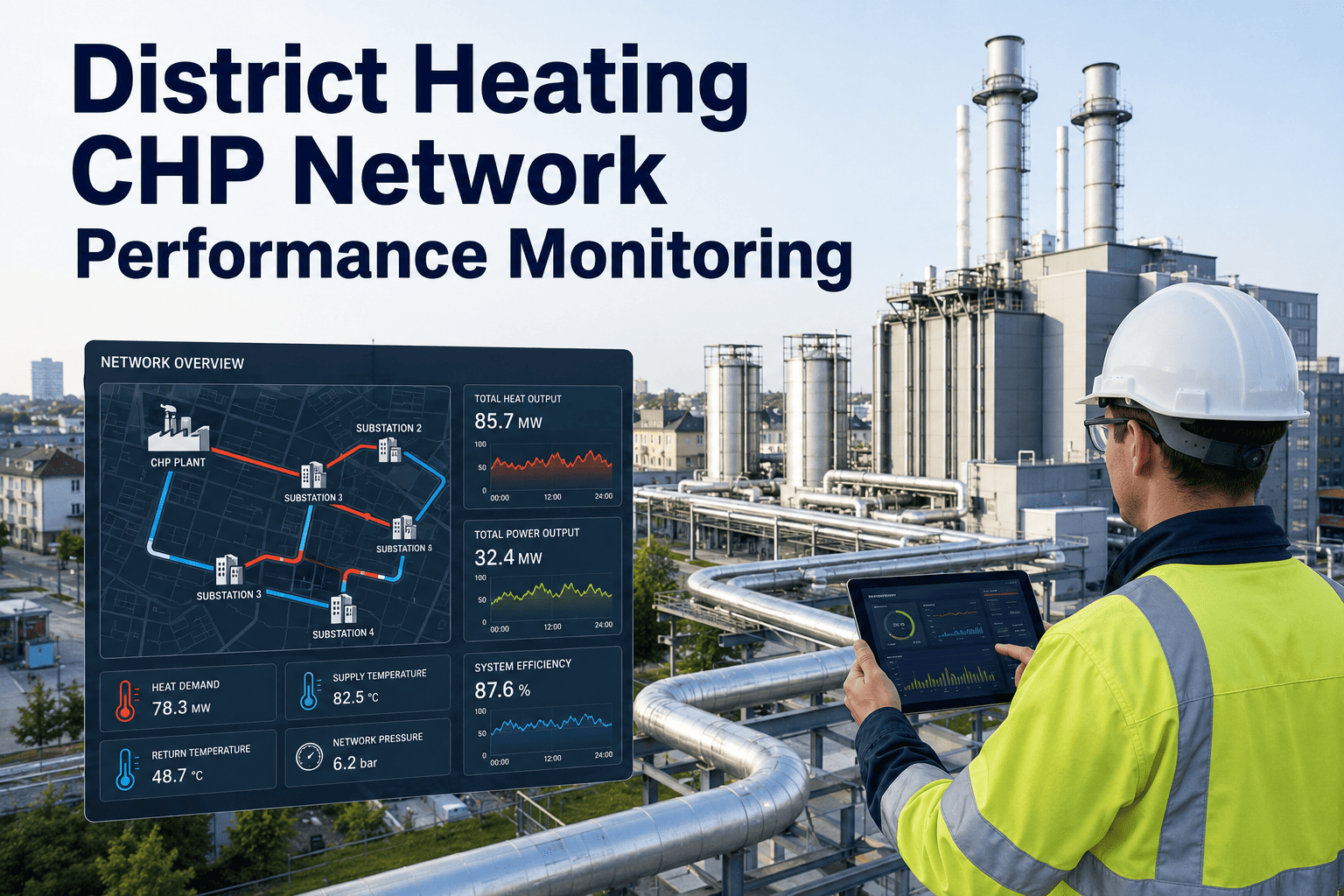
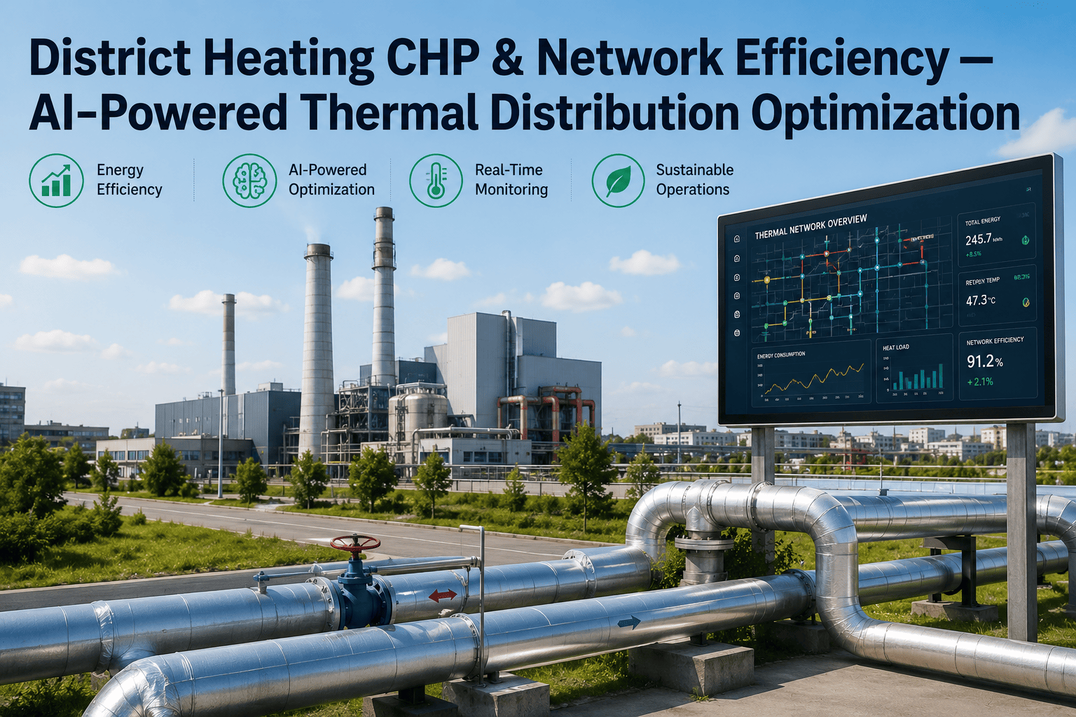
AI-powered thermal distribution optimization for district heating CHP networks monitors supply and return temperatures, flow rates, and heat loss in real time, then adjusts ahead of demand instead of reacting after it — cutting distribution losses without touching combustion efficiency at the plant.
Why CHP Networks Waste Heat Even When the Plant Is Running Efficiently
A combined heat and power plant can hit excellent thermal efficiency at the point of generation and still lose a meaningful share of that heat before it reaches a single radiator. The distribution network — kilometers of buried pipe, pumping stations, and hundreds of building substations — is where efficiency actually gets decided, because every degree of supply temperature above what the network truly needs is a degree radiating into the ground along the entire route. Process engineers who focus purely on CHP unit dispatch and combustion tuning are optimizing the ten percent of the system they can see from the control room, while the other ninety percent quietly gives heat back to the surrounding soil.
The traditional fix — supply temperature curves keyed to outdoor air temperature — is better than a flat schedule but still fundamentally reactive. It responds to what the weather is doing right now, not to what the network will need in the next few hours as building thermal mass, occupancy patterns, and solar gain shift demand around. AI-driven forecasting closes that gap by predicting heat demand ahead of time using weather forecasts, historical consumption patterns, and real-time flow data, then adjusting supply parameters before the demand spike arrives rather than after.
The Four Signals a Network Optimization Model Actually Watches
From Demand Forecast to Supply Adjustment — the Optimization Loop
Want to see where your own network's heat loss is concentrated — by pipe segment, not just as a single network-wide percentage? A 30-minute session can walk through a sample distribution loss breakdown.
Balancing Multiple Energy Sources Without Guesswork
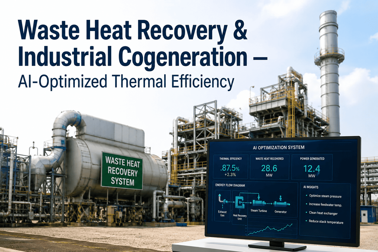
Most modern district heating networks are no longer single-source. A CHP unit anchors baseload, but solar thermal, biomass, or waste heat recovery from an adjacent industrial process may all be feeding the same network at different times of day. Deciding which source to draw from at any given moment — and how much — used to be a manual dispatch decision made against rough rules of thumb. AI optimization treats it as a continuous balancing problem: it weighs the cost-effectiveness and environmental profile of each available source against real-time demand and automatically favors renewable or waste-heat inputs when they can meet the load, reserving CHP output for the gaps those sources can't cover.
This matters for a process engineer's day-to-day work because it removes a category of manual dispatch decisions that previously required constant attention during shoulder seasons, when demand is unpredictable and multiple sources are simultaneously available. The system also supports dynamic pricing models that reflect real-time heat cost, which in turn nudges consumer behavior toward off-peak consumption where that flexibility exists.
Fixed Schedule vs. AI-Optimized Network Control
| Operating Factor | Fixed Weather-Compensation Curve | AI-Optimized Control |
|---|---|---|
| Response to demand shift | Reactive, after outdoor temperature changes | Predictive, ahead of forecasted demand |
| Supply temperature | Set by curve, uniform across network | Continuously calculated to the minimum needed |
| Multi-source dispatch | Manual rules of thumb | Automated, cost and demand weighted |
| Loss visibility | Network-wide estimate | Segment-level, continuously updated |
| Adaptation to new buildings or loads | Requires manual curve recalibration | Model retrains on new consumption data |
Handling the Shoulder Seasons Where Fixed Schedules Struggle Most
Spring and autumn are where fixed weather-compensation curves show their weakest performance, because demand on those days swings hardest within a single 24-hour period — a cold morning followed by a mild, sun-warmed afternoon, followed by a cold evening as buildings lose their solar gain. A curve tuned to the morning's outdoor temperature over-supplies heat by early afternoon, and a curve tuned to the afternoon under-supplies it by evening. This is precisely the pattern that demand forecasting is best at catching, because it incorporates the intra-day shape of the forecast rather than a single outdoor temperature reading, and it's also the period where dispatch between multiple heat sources — solar thermal contributing meaningfully during sunny shoulder-season afternoons, CHP carrying the mornings and evenings — has the most room to reduce cost without sacrificing comfort at the building level.
The same forecasting layer extends naturally into emissions and efficiency compliance reporting, which for a process engineer is often a recurring administrative burden rather than an operational one. Continuous, segment-level logging of supply temperature, return temperature, flow, and calculated heat loss builds the audit trail that regulatory efficiency reporting requires as a byproduct of normal operation, rather than as a separate data-gathering exercise assembled from disconnected SCADA exports each quarter.
What This Looks Like for a Process Engineer on a Normal Week
The practical shift is less about a new control room screen and more about which decisions stop requiring a person. Supply temperature setpoints that used to be adjusted manually in response to a weather forecast are now recalculated continuously and applied automatically, freeing a process engineer's attention for the anomalies that actually need judgment — a substation with a persistently high return temperature suggesting a bypass fault, or a pipe segment showing a heat loss rate that's crept up month over month and might indicate insulation degradation worth investigating before it becomes a bigger repair.
Regulatory and efficiency reporting also becomes less of a manual exercise. Continuous logging of supply, return, flow, and loss data by segment builds the audit trail that efficiency compliance reporting requires, without a process engineer having to assemble it from separate SCADA exports at the end of each reporting period.
Frequently Asked Questions
Does AI optimization require replacing our existing SCADA or DCS system?
No. The optimization layer connects to your existing SCADA, DCS, and flow metering infrastructure as an additional analytics and control-recommendation layer, rather than replacing the control systems you already have in place. Existing supply and return temperature sensors, flow meters, and substation monitoring points feed directly into the model, so the primary integration work is connecting available data streams rather than re-instrumenting the network. Where instrumentation gaps exist at specific substations, additional sensors can be added incrementally rather than as a network-wide retrofit. iFactory Support can walk through compatibility with your specific control system.
How much of the distribution network needs to be instrumented before this works?
Meaningful optimization can start with the instrumentation most networks already have at the plant outlet and major substations — it doesn't require sensors on every meter of pipe on day one. The model identifies which additional monitoring points would most improve loss visibility and demand forecasting accuracy, so instrumentation expansion can be prioritized toward the segments and substations where it delivers the most value first. Coverage typically expands over the first several months of operation as the highest-value gaps are identified from the data already flowing in, rather than as an upfront capital project.
Can this handle a network with multiple heat sources, not just a single CHP plant?
Yes, and multi-source networks are precisely where the optimization has the most to offer. The model treats every available heat source — CHP output, solar thermal, biomass, waste heat recovery — as an input to a continuous dispatch decision, weighing cost, availability, and environmental profile against real-time and forecasted demand. This removes the manual judgment calls that shoulder-season dispatch across multiple sources traditionally required, and it adapts automatically as new sources are added to the network over time rather than needing a full re-configuration.
What kind of heat loss reduction is realistic for an existing network?
The realistic range depends heavily on how far a given network's current operation is from its true minimum supply temperature requirement — a network already running tight weather-compensation curves has less room to improve than one still operating fixed seasonal schedules. What's consistent across networks is that the largest gains come from narrowing the supply-return delta at the substations furthest from the plant, since those are typically where fixed schedules over-supply the most to guarantee adequate heat at the end of the line. A 30-minute assessment of your current supply and return data can give a network-specific estimate rather than a generic industry figure.
How much does the optimization depend on weather forecast accuracy, and what happens when the forecast is wrong?
Weather forecasts are one input among several, not the sole basis for supply decisions, so a forecast miss doesn't leave the network exposed the way a purely forecast-driven schedule might. Real-time flow, supply, and return data are compared against the forecast continuously, and the moment actual conditions diverge from what was predicted, the model corrects supply parameters based on what the network is actually experiencing rather than waiting for the next forecast update. Over time, the model also learns where a given weather forecast source tends to be systematically off — for instance, consistently underestimating wind chill effects on return temperature at exposed substations — and adjusts its own confidence in that input accordingly. The result is a system that degrades gracefully on a bad forecast day rather than one that depends entirely on forecast precision to function.
Every heating season run on a fixed schedule is a season of avoidable loss baked into the network's operating cost. See what your own supply and return data suggests about where that loss is concentrated.