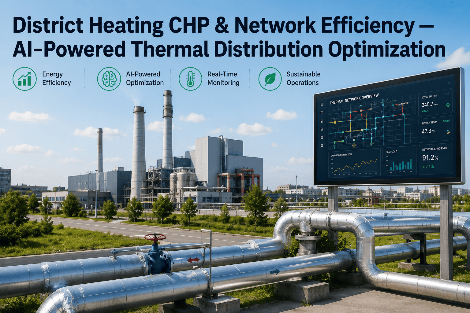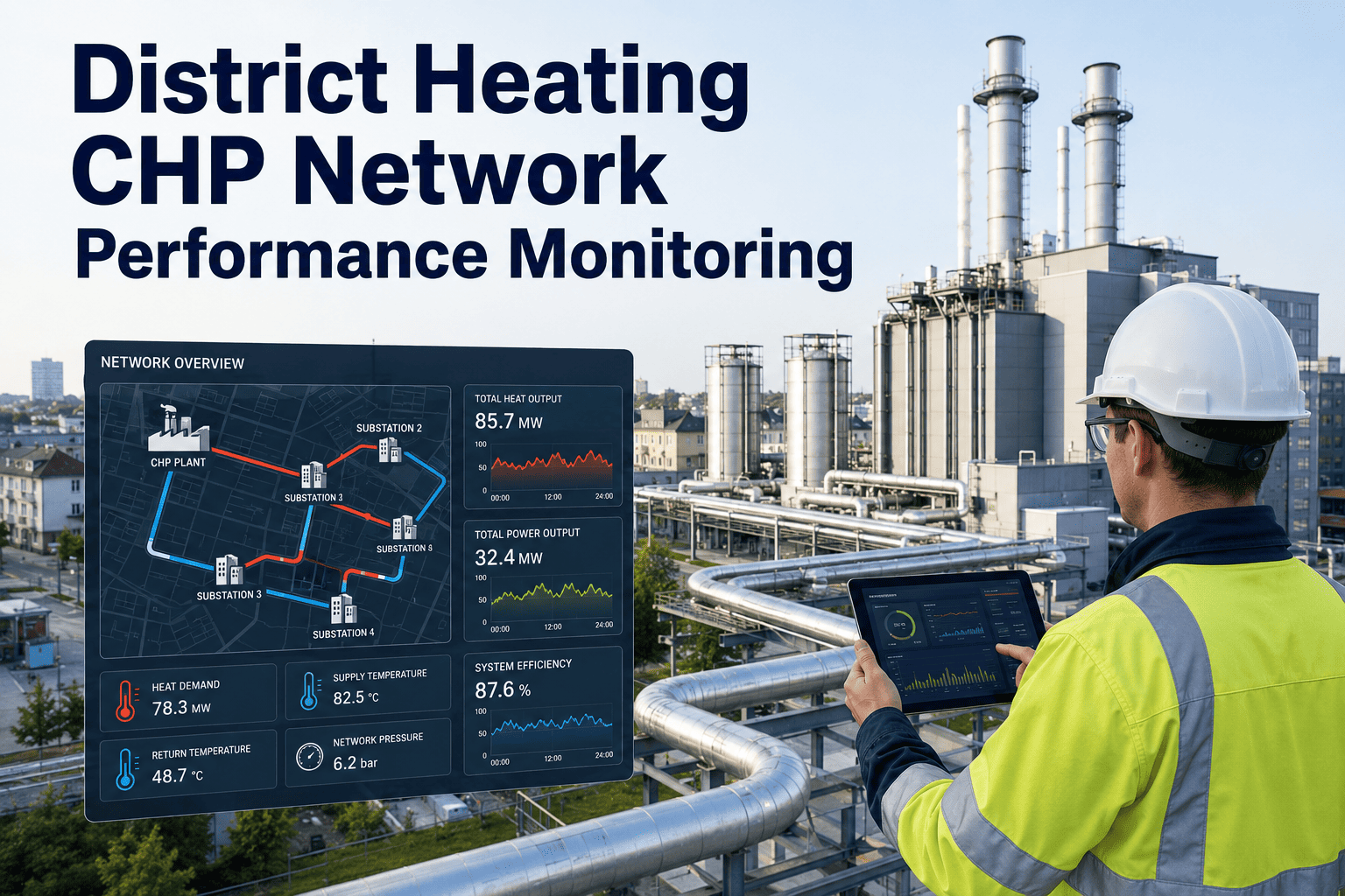
District heating networks powered by combined heat and power plants are engineered to deliver heat efficiently at scale, yet a significant share of generated thermal energy never reaches the consumer. The gap between what the CHP plant produces and what the end user receives is rarely visible in real time, hiding behind monthly settlement reports that average out the peaks and valleys of daily network performance. Operators know their return temperatures run higher than design, that seasonal transitions create demand forecasting blind spots, and that supply temperature setpoints are often adjusted by habit rather than data. What most lack is a continuous, granular view of where heat is being lost across the network and whether their CHP heat-to-power ratio is actually matching real demand. Book a network performance review to see where your CHP district heating system is losing heat you can recover.
Your District Heating Network Is Losing Heat You Cannot Measure
Combined heat and power plants generate thermal energy with high overall efficiency, but the distribution network between the plant and the consumer introduces losses that compound silently. Without segment-level performance monitoring, those losses remain invisible until they appear as excess fuel consumption on the monthly bill.
The Scale of Unmeasured Heat Loss in CHP District Energy
District heating networks are typically monitored at two points: the plant outlet and the aggregate return. Everything that happens in between is inferred, not measured. The result is a system where the majority of thermal losses are detected only indirectly through fuel consumption that exceeds theoretical demand, with no ability to pinpoint where the loss is occurring or what is causing it.
typical total heat loss from CHP plant output to consumer delivery point in networks without segment-level monitoring
average return temperature elevation above design targets across European district heating networks studied in recent benchmarking programs
of network heat loss that occurs in secondary distribution and consumer connections, the segments with the least monitoring coverage
annual fuel consumption reduction reported by networks after implementing continuous segment-level performance monitoring within the first heating season
Where Heat Escapes: A Stage-by-Stage Breakdown
Heat loss is not distributed evenly across a district heating network. Each stage of the distribution chain introduces distinct loss mechanisms, and the cumulative effect means that a significant fraction of the thermal energy generated at the CHP plant never reaches the building it was intended to heat. Understanding where loss concentrates is the first step toward targeting monitoring and maintenance investment where it will have the greatest impact.
CHP Plant Thermal Output
The CHP plant produces thermal energy at the highest efficiency point in the system. At this stage, all generated heat is accounted for through plant-level metering of fuel input, electrical output, and thermal output. The challenge begins the moment this thermal energy enters the distribution network, where measurement granularity drops dramatically compared to the plant itself.
Primary Pipeline Transmission
Primary pipes carry high-temperature water from the CHP plant to district substations, often over distances of several kilometers. Heat loss here is driven by insulation degradation, water ingress into the pipe casing, thermal bridges at fittings and valves, and soil thermal conductivity changes due to groundwater movement. Most networks monitor flow and temperature only at the plant exit and the first substation, making it impossible to isolate which section of primary pipe is responsible for the loss.
District Substation Heat Exchangers
At each substation, heat transfers from the primary network to the secondary network through plate heat exchangers. Losses here come from approach temperature degradation as heat exchanger plates foul, bypass valve leakage that allows hot primary water to flow directly into the return line, and control valve hunting that creates intermittent temperature spikes. Substation performance is typically checked only during annual maintenance, meaning fouling and bypass issues can persist for months before detection.
Secondary Network Distribution
Secondary networks distribute lower-temperature water from substations to individual buildings. These networks often have poorer insulation than primary mains, more frequent fittings and branches, and in older systems may include direct connections that bypass the heat exchanger entirely. Secondary networks are the least monitored segment in most district heating systems, with flow and temperature data rarely available at individual building connections.
Consumer Building Connections
At the building level, losses occur through improperly balanced heating systems that force excess flow, malfunctioning thermostatic radiator valves that cannot modulate properly, and building automation systems that do not communicate demand signals back to the network. In many networks, consumer heat meters are read only for billing purposes, and the data is not fed back into network performance analysis in real time, so building-level imbalances remain invisible to the network operator.
Six Performance Indicators That Reveal Network Health
Monitoring a district heating network effectively requires tracking more than just supply and return temperatures at the plant. The six metrics below provide a comprehensive view of network performance, each exposing a different dimension of heat loss, inefficiency, or demand mismatch that plant-level measurements alone cannot detect.
Measures the gap between the configured supply temperature setpoint and the actual temperature arriving at each substation or consumer connection. Persistent positive deviation indicates over-supply, which wastes fuel and stresses pipe insulation. Negative deviation indicates under-supply, which triggers consumer complaints and can cause comfort problems in downstream buildings.
Tracks how much the return temperature at each network segment exceeds its design target. Elevated return temperature is the single most common indicator of network inefficiency, signaling bypass flows, improperly balanced substations, consumer-side control failures, or direct connections that dump heat into the return line without delivering it to the building.
The difference between supply and return temperature at any point in the network. Design delta T is typically 30 to 40 degrees for low-temperature networks, but real-world delta T is often compressed to 20 to 25 degrees. Every degree of compression means the same volume of water carries less heat, forcing higher flow rates and increasing pumping energy consumption proportionally.
Calculated as the difference between thermal energy entering a network segment and thermal energy leaving it, expressed as a percentage of the entering energy. This metric isolates actual distribution losses from production-side inefficiencies and reveals which specific pipe sections or substations are responsible for the largest share of total network loss.
Compares the actual heat-to-power ratio the CHP plant is operating at against the ratio that would optimally match current network demand. When the plant produces more heat than the network can absorb efficiently, or less heat than needed, the ratio drift indicates a mismatch between generation scheduling and real-time demand that is costing fuel or requiring supplemental boiler firing.
The percentage difference between predicted heat demand and actual heat demand over a rolling window. High forecast error forces the CHP plant to operate in a reactive mode, increasing start-stop cycles, reducing average electrical efficiency, and making it impossible to maintain the optimal heat-to-power ratio. Persistent forecast error also undermines operator confidence in automated control systems.
Turn Invisible Losses Into Measurable Improvements
Segment-level monitoring connects to your existing SCADA infrastructure, calculates per-segment performance metrics in real time, and surfaces the specific locations where your district heating network is losing thermal energy you are paying to generate.
Supply and Return Temperature: The Diagnostic Pair
Supply and return temperatures are not independent variables in a district heating network. They form a coupled system where deviation in one inevitably drives deviation in the other. Understanding how they interact, and what specific network conditions cause each to deviate from design, is the foundation of effective network performance management.
Supply temperature is routinely set higher than design to compensate for perceived delivery problems, most commonly elevated return temperatures that reduce the effective heat transfer at consumer substations. Raising supply temperature does solve the immediate comfort complaint, but it increases heat loss from primary pipes proportionally, degrades pipe insulation faster due to sustained higher operating temperatures, and creates a feedback loop where higher supply temperatures push return temperatures even higher as excess heat dumps into the return through bypass flows and consumer-side imbalances. Networks that measure supply temperature only at the plant outlet cannot see how much of this over-supply is actually reaching substations versus being lost in transit.
Elevated return temperature is the most widespread and most expensive efficiency problem in district heating. It indicates that water is returning to the plant carrying heat it was supposed to deliver to buildings but did not. The causes range from stuck bypass valves at substations that short-circuit the heat exchanger, to consumer buildings with improperly balanced hydronic systems that cannot extract the available heat, to direct connections where primary network water circulates through building radiators without a heat exchanger and returns at temperatures far above the design target. Every degree of return temperature elevation above design typically costs one to two percent of total fuel consumption, making it the highest-leverage single metric to improve.
When supply temperature runs 12 degrees above design and return temperature runs 15 degrees above design, the delta T compresses from the designed 37 degrees down to as little as 10 degrees in the worst cases. This compression means the network must circulate nearly four times the design flow volume to deliver the same amount of heat. The consequences cascade through the entire system: pumping energy increases proportionally with flow, pipe velocities approach or exceed design limits causing erosion and noise, and the CHP plant must produce more thermal energy per unit of delivered heat, reducing both fuel efficiency and electrical cogeneration output. Restoring design delta T is not a marginal improvement, it is a structural correction that unlocks capacity across the entire network.
Network Segment Heat Loss Breakdown
Heat loss distribution varies significantly across network segments, and most operators only measure total loss at the plant boundary rather than at each stage. The table below shows typical loss ranges by segment, the primary physical mechanism driving that loss, and the monitoring gap that allows it to persist undetected in conventional network management approaches.
The critical insight is that secondary networks and consumer connections, which together account for the largest share of loss, are typically the least monitored segments. A monitoring system that only tracks supply and return at the plant level cannot distinguish whether elevated return temperature originates from primary pipe losses, substation inefficiency, or secondary network problems. Segment-level monitoring closes that gap and directs maintenance investment where it will have the greatest impact on overall network efficiency and fuel consumption.
Why Demand Forecasting Fails in Most CHP Heating Networks
Accurate demand forecasting is essential for CHP plants because the heat-to-power ratio is physically constrained by the generation equipment. When the forecast is wrong, the plant either over-generates heat and wastes fuel or under-generates and must fire supplemental boilers at lower efficiency. The following five failures explain why most district heating demand forecasts carry error rates of 15 to 25 percent when they need to be below 10 percent for effective CHP optimization.
Weather Data Resolution Too Coarse for Network Response Time
Most demand forecasting models rely on ambient temperature forecasts from weather services, typically available at one-hour resolution. District heating networks respond to temperature changes on a much shorter timescale, and the thermal inertia of the network means that production adjustments made now will not reach consumers for 30 to 90 minutes depending on network size and flow velocity. This mismatch between forecast granularity and network response time creates systematic overproduction during cooling trends and underproduction during warming trends that never averages out because the errors are directionally consistent within each weather pattern.
Building Thermal Inertia Not Modeled
Buildings do not respond instantaneously to changes in outdoor temperature. The thermal mass of concrete, brick, and internal furnishings creates a lag of several hours between a temperature change outside and a corresponding change in heating demand inside. Forecasting models that map outdoor temperature directly to heat demand without accounting for this thermal lag will consistently over-predict demand during cold fronts arriving after warm periods and under-predict demand during cold fronts arriving after already-cold periods. The error can reach 20 to 30 percent during seasonal transitions when thermal lag effects are largest.
Solar Gain and Internal Loads Excluded
Modern buildings with good insulation and large window areas can experience significant solar heat gain that reduces or eliminates heating demand during daytime hours even in winter. Internal loads from occupants, equipment, and lighting add further variability that is completely invisible to a forecasting model based only on outdoor temperature. In well-insulated buildings, solar gain and internal loads can account for 30 to 50 percent of the total heat balance during daytime hours, making their omission a major source of forecast error during midday periods when the CHP plant may be over-producing heat that the network cannot absorb.
No Network Condition Input to Forecast Model
The same weather conditions produce different heat demand depending on the current state of the network. A network with elevated return temperatures due to a partially failed substation will require higher supply temperatures to meet the same consumer demand, which changes the relationship between outdoor temperature and plant-level heat demand. Similarly, a network that has lost insulation integrity in a major pipe section will show higher apparent demand for the same weather conditions because more heat is being lost in transit. Forecasting models that do not receive real-time network condition data as an input variable cannot account for these state-dependent demand shifts.
Base Load and Variable Load Not Separated
District heating demand consists of a base load component driven by domestic hot water use and a variable component driven by space heating response to outdoor temperature. These two components follow fundamentally different patterns: base load is relatively flat with minor peaks in morning and evening, while variable load follows a smooth curve driven by outdoor temperature with a thermal lag. Forecasting models that treat total demand as a single variable rather than decomposing it into base and variable components will misestimate both, particularly during shoulder seasons when the ratio between base and variable demand shifts rapidly and the model lacks the structural flexibility to track both components independently.
What Changes With Continuous Network Performance Monitoring
Figures from typical deployments across district heating networks with CHP supply within the first two heating seasons after implementing continuous segment-level monitoring and automated performance analytics.
A Network Operations Manager on Finding the Lost Heat
We had been running our CHP plant at a fixed heat-to-power ratio for three years because we had no real-time visibility into what the network actually needed. Once we installed segment-level monitoring, we discovered that our return temperature was twelve degrees above design during shoulder months because half our substations had bypass valves that were stuck partially open. We were essentially heating the ground between the plant and the consumers. Fixing those bypass valves and adjusting our supply temperature curve based on actual substation return data reduced our fuel consumption by eight percent in the first heating season alone, and we finally had the data to justify the maintenance backlog we had been unable to prioritize before.
Frequently Asked Questions
What is the ideal delta T for a district heating network, and why does it matter?
The ideal delta T depends on the network design temperature regime, but for a typical low-temperature district heating network designed for 80 degrees Celsius supply and 45 degrees Celsius return, the target delta T is 35 degrees. In practice, many networks operate with a delta T of 20 to 25 degrees due to elevated return temperatures, which means the same volume of water is carrying significantly less heat than designed. Every degree of delta T compression forces the network to pump more water to deliver the same thermal energy, increasing electrical pumping costs and reducing the effective capacity of existing pipes. Book a demo to see how delta T tracking works across your network segments.
How frequently should supply temperature setpoints be adjusted during the heating season?
Supply temperature setpoints should ideally be adjusted continuously based on real-time demand signals rather than on fixed seasonal curves or operator judgment. Modern network performance monitoring systems use outdoor temperature, forecasted demand, and real-time return temperature data to calculate the optimal supply temperature every 15 to 30 minutes. Networks that still adjust setpoints once or twice per day, or once per season, are consistently over-supplying heat during mild periods and under-supplying during cold snaps, with fuel waste typically ranging from five to fifteen percent. Talk to a specialist about automating your supply temperature control logic.
Can network performance monitoring integrate with existing SCADA systems?
Yes, segment-level monitoring data can integrate with existing SCADA systems through standard industrial protocols including OPC UA, Modbus TCP, and REST APIs. The monitoring layer sits alongside your SCADA system and enriches it with calculated performance metrics that most SCADA platforms are not designed to compute, such as per-segment heat loss rates, delta T compression factors, and demand forecast accuracy scores. Integration does not require replacing your existing SCADA infrastructure but rather feeding additional structured data into it. Book a demo to see integration options for your current SCADA platform.
What is the typical payback period for segment-level monitoring in a district heating network?
The payback period for segment-level monitoring in a district heating network typically ranges from six to eighteen months depending on network size, current heat loss levels, and fuel costs. Networks with high return temperatures and poorly understood loss distribution tend to see the fastest payback because the monitoring immediately identifies specific, actionable maintenance tasks that reduce fuel consumption. A mid-size network consuming 50 GWh of heat annually that reduces losses by three percentage points saves 1.5 GWh per year, which at typical European gas prices translates to rapid return. Talk to a specialist to model the payback for your specific network configuration.
How does continuous monitoring reduce CHP fuel consumption in practice?
Continuous monitoring reduces CHP fuel consumption through three primary mechanisms: enabling dynamic supply temperature optimization that eliminates habitual over-supply, identifying specific network segments with elevated losses so maintenance can be targeted rather than generalized, and providing the real-time demand visibility needed to adjust the CHP heat-to-power ratio to match actual demand. Networks that implement continuous monitoring typically report fuel savings of five to twelve percent in the first full heating season, with additional savings accumulating as the data drives targeted improvements over subsequent years. Book a demo to see the fuel savings model applied to your CHP configuration.
The Bottom Line on CHP District Heating Network Performance
The gap between CHP thermal output and heat delivered to consumers is not an abstraction, it is a measurable, segment-by-segment reality that most district heating networks do not monitor in real time. Elevated return temperatures compress delta T and force higher flow rates for the same heat delivery. Supply temperature setpoints that are adjusted by routine rather than by real-time data consistently over-supply the network during mild weather and under-supply during cold snaps. Demand forecasting models that ignore network thermal inertia and segment-level losses produce errors that cascade into CHP operational decisions, wasting fuel and accelerating equipment wear. Undetected heat losses in secondary networks and at consumer connections represent the largest single category of loss in most systems, yet these segments receive the least monitoring attention. A monitoring approach that tracks performance at each network segment, connects those measurements to substation condition data, and feeds real-time demand signals back into CHP control logic transforms the network from a passive distribution system into an actively managed thermal grid where fuel savings, reduced maintenance costs, and extended infrastructure life typically justify the investment within the first heating season.
Stop Paying for Heat That Never Reaches a Building
Book a 30-minute network performance review. Bring your current supply and return temperature data and recent fuel consumption records, and iFactory will map your loss distribution across network segments and scope a monitoring rollout calibrated to your CHP configuration.