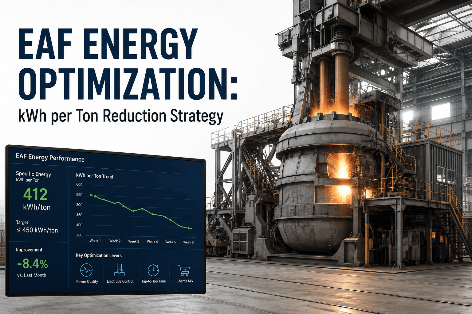
Electric arc furnaces consume between 380 and 550 kilowatt-hours per ton of liquid steel, making the EAF the single largest energy consumer in any mini-mill or EAF-based steelmaking operation. A 10 kWh per ton reduction across a two-million-ton annual operation translates to 20 million kWh saved per year, which at industrial electricity rates represents two to four million dollars in direct energy cost reduction depending on the utility region. Despite this magnitude of opportunity, most EAF energy optimization efforts remain fragmented, addressing individual variables like power profile or oxygen injection in isolation rather than as an integrated system where every parameter interacts with every other parameter in real time. The plants that achieve the lowest sustained kWh per ton numbers are not using secret technology. They are applying systematic optimization across all energy-consuming subsystems simultaneously, supported by real-time data analytics that measure the impact of every adjustment. To see how integrated EAF energy analytics works in practice, Book a Demo with the iFactory AI steelmaking team.
EAF Energy Optimization — Systematic kWh per Ton Reduction Strategy
iFactory AI delivers integrated EAF energy analytics covering power profile tuning, oxygen and gas injection optimization, foamy slag management, and scrap preheating impact measurement for sustained kWh per ton reduction.
Where EAF Energy Actually Goes — The Distribution That Defines Your Optimization Targets
Effective energy optimization requires understanding exactly where electrical energy is consumed within the EAF process, because each consumption category has a different optimization lever and a different maximum reduction potential. The energy that reaches the liquid steel as sensible heat is typically only 55 to 65 percent of total electrical input. The remaining 35 to 45 percent is distributed across losses that are partly unavoidable thermodynamics and partly addressable through operational adjustments. The visual breakdown below maps the typical energy distribution for a modern high-power EAF, providing the structural reference for where optimization efforts should be directed and what magnitude of savings is realistically achievable in each category.
The useful energy that raises scrap and direct reduced iron from ambient temperature to tap temperature, approximately 1,600 to 1,650 degrees Celsius. This is the energy you cannot reduce without changing the fundamental thermodynamics of steelmaking. However, the input required to deliver this energy can be reduced by improving the efficiency of the heat transfer mechanisms, particularly foamy slag practice and arc stability.
Optimization Lever: Improve heat transfer efficiency to reduce input needed for same outputEnergy consumed heating the slag layer to liquidus temperature and maintaining it throughout the heat. Slag mass is directly proportional to the scrap quality and the amount of oxidation products generated during melting. Higher residual elements in scrap produce more slag, consuming more energy that does not contribute to steel heating. Optimizing slag practice means reducing unnecessary slag mass while maintaining the foamy slag layer needed for arc shielding.
Optimization Lever: Minimize slag mass through scrap mix control and oxidation managementHeat extracted by the water-cooled panels, delta sections, and roof. Some of this cooling is essential for panel integrity, but excessive cooling represents energy that was paid for and then deliberately removed from the furnace. The balance between sufficient cooling for refractory and panel protection and excessive cooling that wastes energy is one of the most under-optimized parameters in EAF operations. Panels that run too cold are removing energy that should be heating steel.
Optimization Lever: Optimize cooling water flow and temperature to minimize unnecessary heat extractionEnergy carried out of the furnace by the off-gas stream, primarily as sensible heat in CO, CO2, and entrained particulate. The off-gas temperature at the furnace elbow typically ranges from 1,200 to 1,500 degrees Celsius, representing substantial energy content. Scrap preheating systems attempt to recover a portion of this energy, but even without preheating, optimizing the off-gas flow rate and composition reduces the energy lost per ton of steel. Lower CO content in off-gas means more complete combustion and less chemical energy leaving the furnace.
Optimization Lever: Optimize post-combustion and off-gas flow to minimize chemical and thermal lossesLosses in the transformer, flexible cables, bus tubes, and electrode column before energy reaches the arc. These losses are partly fixed by the electrical infrastructure design but are influenced by the operating power factor, the electrode position relative to the furnace shell, and the secondary voltage tap selection. Operating at a lower power factor than necessary increases I-squared-R losses in the secondary system, consuming energy that never reaches the arc. Optimizing tap selection and maintaining electrode column alignment reduces these avoidable losses.
Optimization Lever: Optimize tap selection and power factor to minimize secondary circuit lossesRadiation losses through openings including the slag door, electrode ports, and any gaps in the roof seal. These losses are highly sensitive to door management practices, roof condition, and the time spent with the furnace in open positions during charging and tapping. While individual radiation events are brief, their high rate of energy loss means that cumulative radiation during door-open time can represent a meaningful share of total energy consumption per heat. Tight door management and rapid roof closure after charging directly reduce this loss category.
Optimization Lever: Minimize open-furnace time through rapid charging and door management disciplinePower Profile Optimization — The Highest-Impact Single Lever for kWh Reduction
The power profile defines how electrical power is applied to the EAF throughout the heat, specifying the tap position, impedance setpoint, and arc length at each stage from bore-down through flat bath to refine and tap. Most EAFs operate on a static power profile that was established during commissioning and has been adjusted incrementally over years of operation, often without systematic analysis of whether the profile still matches the current scrap mix, furnace condition, and production requirements. Power profile optimization does not mean simply running at higher power. It means applying the right amount of power at the right arc length at each stage to maximize the fraction of electrical energy that transfers as heat to the steel rather than being lost to radiation, off-gas, or panel cooling. The phase breakdown below maps the power profile optimization opportunity at each stage of the heat.
Long Arc, High Voltage, Controlled Power
During initial bore-down, the scrap forms a cave structure that shields the furnace sidewalls from direct arc radiation. This is the phase where long arc operation with higher voltage and lower current is most efficient because the scrap cage protects the panels while the long arc penetrates deep into the charge. The optimization opportunity is to maximize voltage during this phase while monitoring for cave-in events that could expose the sidewall. Many operations reduce voltage too early out of caution, leaving 5 to 10 kWh per ton on the table by not exploiting the natural sidewall protection that the scrap cage provides during the first minutes of the heat.
Typical Savings: 5–10 kWh/ton from extended high-voltage bore-downDynamic Arc Length Management
As the scrap cave collapses and the bath begins to form, the sidewall protection disappears and arc length must be reduced to prevent panel damage. This is where the most sophisticated power profile optimization occurs, because the optimal arc length changes continuously as the scrap-to-liquid ratio shifts. Fixed impedance setpoints that were correct at minute eight are suboptimal by minute fifteen. AI-driven dynamic impedance adjustment that responds to the real-time scrap melt state, detected through electrode position, power fluctuations, and off-gas temperature changes, can reduce energy consumption by 8 to 15 kWh per ton during this phase alone by maintaining the optimal balance between arc length for heat transfer efficiency and arc length for panel protection.
Typical Savings: 8–15 kWh/ton from dynamic impedance during meltingFoamy Slag Submersion and Power Maximization
Once a flat bath is established, the primary optimization objective is to submerge the arc completely in foamy slag so that maximum power can be applied without radiation damage to sidewalls. Foamy slag quality directly determines how much power can be pushed during this phase. Slag that is too thin or unstable forces a power reduction to protect panels, extending tap-to-tap time and increasing kWh per ton through prolonged heat losses. The optimization lever here is not the power profile itself but the foamy slag practice that enables the power profile to deliver its full potential. Plants that achieve consistent 300 to 400 millimeter foamy slag depth can run 15 to 20 percent higher power during flat bath compared to plants with inconsistent slag practice.
Typical Savings: 5–12 kWh/ton from foamy slag-enabled power maximizationMinimum Energy Temperature Adjustment
The final phase should be as short as possible because additional energy input during refining is the least efficient use of electrical power in the EAF. Every minute spent superheating beyond the target tap temperature is wasted energy because the steel will lose temperature during tapping and transfer anyway. The optimization target is to arrive at flat bath within 10 to 15 degrees of tap temperature so that the refine phase requires minimal energy for final adjustment. This is achieved through accurate temperature prediction at the flat bath stage, allowing the melting phase to target the correct endpoint rather than overshooting and then holding at temperature or undershooting and requiring extended refining.
Typical Savings: 3–8 kWh/ton from minimized refining timeChemical Energy Optimization — Oxygen, Gas, and Carbon Injection Balance
Chemical energy from oxygen lancing, natural gas injection, and carbon injection typically contributes 25 to 35 percent of total energy input to the EAF heat. This chemical energy is cheaper per unit than electrical energy in most utility regions, which creates a strong economic incentive to maximize the chemical-to-electrical energy ratio. However, chemical energy injection is not free energy. Excessive oxygen increases slag volume and iron oxidation losses, excessive carbon injection without matching oxygen produces soot and incomplete combustion that exits through the off-gas system, and unbalanced gas injection can destabilize the foamy slag layer. The optimization challenge is finding the balance point where chemical energy displaces the maximum amount of electrical energy without creating secondary costs that exceed the energy savings. The interaction matrix below maps how each chemical energy input affects the key process variables that determine overall energy efficiency.
| Input Variable | Increase Effect on Heat Input | Increase Effect on Slag Volume | Increase Effect on Iron Yield | Increase Effect on Foamy Slag | Optimization Risk if Excessive |
|---|---|---|---|---|---|
| Oxygen Lancing | Direct: exothermic Fe and C oxidation | High: more FeO in slag | Negative: Fe oxidation to slag | Positive: CO generation for foam | Yield loss exceeds energy value above 35–40 Nm3/t |
| Natural Gas Injection | Direct: combustion enthalpy | Low: minimal slag contribution | Neutral: no direct Fe interaction | Moderate: additional CO2 and H2O for foam | Off-gas temperature spike if not absorbed by slag |
| Carbon Injection | Indirect: provides fuel for foamy slag CO generation | Low: carbon dissolves or reacts | Negative if excess: carburization beyond spec | High: primary foam generator with oxygen | Over-foaming, carbon pickup exceeding limits |
| Post-Combustion O2 | Indirect: combusts CO to CO2 in freeboard | Moderate: additional FeO from CO2 | Slightly negative: some Fe re-oxidation | Low: acts above slag surface | Panel overheating if combustion zone contacts sidewall |
Foamy Slag as an Energy Optimization Tool, Not Just a Practice Requirement
Most EAF operators understand foamy slag as a necessary practice for arc shielding and panel protection. Fewer treat it as an energy optimization tool with quantifiable impact on kWh per ton. The energy impact of foamy slag operates through three mechanisms that are often discussed separately but must be managed as an integrated system. First, arc submersion in slag increases the fraction of arc energy transferred to the bath by 15 to 25 percent compared to an exposed arc, because the slag absorbs radiation that would otherwise hit the sidewalls and transfers it to the steel through conduction and convection. Second, foamy slag acts as thermal insulation on the bath surface, reducing heat losses to the off-gas by 10 to 15 percent compared to an open bath surface. Third, consistent foamy slag enables higher sustained power input during flat bath, reducing the time the furnace spends at lower power levels where fixed losses per minute consume a larger share of total energy input. The diagnostic checklist below identifies the most common foamy slag deficiencies that limit energy optimization and the corrective adjustments that address each one.
Quantifying Scrap Preheating Contribution to kWh per Ton Reduction
Scrap preheating systems, whether shaft-type preheaters, Consteel-type continuous conveyors, or bucket preheating systems, recover thermal energy from the EAF off-gas to raise the scrap temperature before it enters the furnace. The energy savings from preheating are directly measurable as a reduction in electrical energy input because each degree of preheat temperature reduces the sensible heat that must be supplied electrically. However, the actual savings achieved in practice frequently fall below the theoretical potential because of heat losses in the preheating system, inconsistent scrap temperature distribution, and the interaction between preheated scrap and other process parameters like charge timing and slag formation. The measurement framework below provides a method for quantifying the actual electrical energy reduction attributable to scrap preheating, separating it from concurrent improvements in other optimization areas that might otherwise be credited to preheating.
Shaft preheaters typically achieve 200 to 400 degrees Celsius preheat on the first charge, while Consteel systems achieve 400 to 600 degrees on continuously fed scrap. Bucket preheating is limited to 50 to 200 degrees due to heat distribution constraints within the bucket. The electrical energy saving is approximately 0.35 kWh per ton per degree Celsius of average preheat temperature across the entire charge.
Based on the specific heat of steel and the preheat temperature achieved, the theoretical electrical energy displacement ranges from 15 kWh per ton for low-temperature bucket preheating to 30 kWh per ton for high-temperature shaft or Consteel preheating. This is the maximum saving achievable if all preheated energy reaches the steel without losses in the preheating system or the EAF itself.
Accounting for heat losses in the preheater, uneven temperature distribution in the scrap charge, and the fact that not all charge material passes through the preheater on every heat, the realistic achievable saving is typically 65 to 75 percent of the theoretical value. Plants reporting 30 kWh per ton savings from preheating are almost certainly including concurrent optimization improvements in their calculation. For measurement methodology guidance, Book a Demo with iFactory AI.
Preheated scrap reduces the time the arc operates against cold scrap, which is the phase of highest electrode oxidation and tip consumption. Plants with effective scrap preheating consistently report 5 to 8 percent reduction in electrode consumption per ton, adding a secondary cost benefit that is not captured in the kWh per ton metric but contributes to overall cost per ton improvement.
The Correct Sequencing of EAF Energy Optimization Initiatives
One of the most common mistakes in EAF energy optimization is pursuing multiple initiatives simultaneously without establishing the contribution of each. When power profile changes, oxygen injection adjustments, and slag practice modifications are all implemented in the same period, the resulting kWh per ton improvement cannot be attributed to any specific lever, which makes it impossible to know which initiatives are delivering value and which are adding cost without benefit. The correct approach is a sequential deployment where each optimization is isolated, measured, and validated before the next is introduced. The sequencing roadmap below defines the recommended order based on the typical magnitude of savings, the complexity of implementation, and the dependency relationships between optimization levers.
Establish Measured kWh per Ton Baseline With Heat-Level Resolution
Before changing anything, install or validate the energy measurement infrastructure to capture total electrical energy input per heat, tap weight, and tap temperature for every heat over a minimum four-week baseline period. The baseline must be stable, meaning the standard deviation of kWh per ton is consistent and not declining due to an unidentified concurrent improvement. Without a stable baseline, every subsequent optimization claim is indefensible. The baseline must also segment kWh per ton by scrap mix category because scrap variation is the largest confounding variable in EAF energy analysis.
Optimize Power Profile With All Other Parameters Held Constant
Adjust the power profile including tap schedule, impedance setpoints, and arc length targets while holding oxygen injection, carbon injection, and scrap mix constant. Run the optimized profile for a minimum of 100 heats to establish statistical significance against the baseline. Measure the kWh per ton change and the tap-to-tap time change independently because power profile changes often affect both. This step typically delivers 15 to 25 kWh per ton reduction and is the highest-impact single initiative in most EAF operations.
Stabilize Foamy Slag to Enable Sustained High Power During Flat Bath
With the optimized power profile in place, improve foamy slag consistency to allow the flat bath power level to be maintained or increased. Measure the impact on kWh per ton separately from the power profile impact by comparing heats with good slag practice against heats with poor slag practice while running the same power profile. This step typically delivers an additional 5 to 12 kWh per ton and also reduces panel wear rates, which is a secondary benefit that should be quantified separately.
Rebalance Oxygen, Gas, and Carbon for Maximum Electrical Displacement
With stable power profile and foamy slag, adjust chemical energy inputs to displace electrical energy while monitoring iron yield, tap carbon, and slag volume. The optimization target is the chemical-to-electrical energy ratio that minimizes total cost per ton, not just kWh per ton, because chemical energy has a different cost structure and yield impact than electrical energy. This step requires careful multivariable analysis because changing oxygen rate affects slag, which affects foamy slag, which affects the power profile that was optimized in step two. For multi-variable optimization support, contact iFactory Support.
Measure Scrap Preheating Contribution With All Other Variables Controlled
If a scrap preheating system is in place or being considered, measure its contribution only after steps one through four are stable. Compare heats with preheating active against consecutive heats with preheating bypassed, holding all other parameters constant. This isolation is essential because preheating interacts with almost every other variable: it changes scrap density, affects slag formation timing, and alters the initial bore-down behavior that the power profile was tuned for. The measured preheating benefit is almost always lower than the theoretical value, and knowing the actual number prevents over-investment in preheating capacity.
Aggregated EAF Energy Optimization Results Across Steelmaking Operations
The performance metrics below reflect measured outcomes from structured EAF energy optimization programs where the sequential methodology described above was followed, allowing each initiative to be measured in isolation before the next was introduced. These figures represent the realistic achievable range for each optimization lever when implemented with proper measurement discipline, as opposed to the inflated savings claims that result from attributing all improvements to a single initiative. The cumulative savings from executing all five steps sequentially typically falls in the 35 to 55 kWh per ton range, which at 2025 industrial electricity rates represents five to twelve dollars per ton in energy cost reduction.
Savings from extended high-voltage bore-down, dynamic impedance during melting, and minimized refining time. Largest single- lever reduction in most operations, achievable within 6 to 8 weeks of structured tuning.
Savings from improved arc submersion, reduced radiation losses, and enabled higher flat bath power. Requires 4 to 6 weeks of slag practice adjustment and carbon-oxygen ratio tuning.
Electrical displacement from optimized oxygen, gas, and carbon injection. Net savings after accounting for yield impact and slag volume changes, requiring 8 to 12 weeks of multivariable testing.
Measured electrical reduction from active preheating versus bypass, net of system heat losses. Range reflects preheater type from bucket to shaft. Capital-intensive with 2 to 5 year payback.
EAF Energy Optimization — FAQs for Steelmaking Engineers and Managers
What is a realistic total kWh per ton reduction target for a typical EAF operation?
For an EAF operation currently consuming between 420 and 480 kWh per ton with no systematic optimization program in place, a realistic total reduction target over a 12 to 18 month program is 35 to 55 kWh per ton. This assumes sequential implementation of power profile optimization, foamy slag stabilization, and chemical energy rebalancing, with or without scrap preheating depending on the installed equipment. Operations already below 400 kWh per ton will find it progressively harder to achieve additional reductions because the remaining losses are increasingly dominated by thermodynamic minimums rather than operational inefficiencies. Operations above 500 kWh per ton typically have the largest headroom for improvement, often 50 to 80 kWh per ton, because high consumption usually indicates multiple simultaneous inefficiencies that compound each other. To establish your specific reduction potential, Book a Demo for a baseline assessment.
How do we separate energy savings from power profile changes versus scrap mix changes?
Scrap mix variation is the single largest confounding variable in EAF energy analysis. The only reliable method is to segment kWh per ton data by scrap mix category and compare within categories, not across them. If the scrap mix changes from 80 percent heavy melt to 60 percent heavy melt and 20 percent turnings, the kWh per ton will increase by 15 to 25 kWh per ton regardless of any power profile changes. If a power profile optimization was implemented simultaneously, the actual savings are masked unless the data is segmented. The analytical approach is to define three to five scrap mix categories based on bulk density and residual content, establish separate baselines for each, and measure optimization impact within each category independently. For scrap-segmented analytics setup, reach out through iFactory Support.
Does power profile optimization increase electrode consumption?
It depends on the direction of the change. Extending high-voltage bore-down can increase electrode tip consumption slightly during the early phase because longer arcs produce more electrode tip exposure to the arc environment. However, this is typically offset by reduced electrode consumption during the melting and flat bath phases because the optimized profile reduces total heat time, which reduces the total time electrodes are exposed to oxidation. Net electrode consumption change from a well-executed power profile optimization is typically between negative 2 percent and positive 3 percent, meaning it is approximately cost-neutral on electrodes while delivering significant electrical energy savings. If electrode consumption increases by more than 5 percent after a power profile change, the profile was likely too aggressive on voltage during phases where the sidewall protection was insufficient and the arc was radiating directly onto electrodes as well as panels.
How quickly can we expect to see measurable kWh per ton improvement after changing the power profile?
A properly designed power profile change should produce a measurable shift in the kWh per ton distribution within 20 to 30 heats, which at typical EAF production rates means three to five days. However, establishing statistical confidence that the shift is real and sustainable requires a minimum of 100 heats under the new profile, which is typically two to three weeks. During this validation period, it is essential that no other significant process changes are introduced, or the attribution becomes ambiguous. The most common mistake is declaring success after 20 heats and then introducing a concurrent oxygen adjustment that either amplifies or masks the power profile effect, making it impossible to determine the true contribution of either change. Patience during the 100-heat validation window is the discipline that separates credible optimization programs from wishful thinking.
What is the minimum data infrastructure needed to start EAF energy optimization?
The minimum data infrastructure for credible EAF energy optimization includes three data streams sampled at one-second resolution or better: total active power input to the furnace in kilowatts, cumulative energy consumption per heat in kilowatt-hours, and tap weight per heat in tons. With these three data streams, you can calculate kWh per ton for every heat and begin identifying the variation that reveals optimization opportunities. Additional data streams that dramatically improve optimization quality include per-phase current and voltage for impedance analysis, oxygen and carbon injection flow rates, off-gas temperature and composition, and cooling water flow and temperature rise for heat loss calculation. The iFactory AI EAF analytics platform connects to these data streams through standard industrial protocols and produces the heat-level and phase-level energy analysis needed to drive the sequential optimization methodology. For a data readiness assessment, Book a Demo with our steelmaking engineering team.
Reduce Your EAF kWh per Ton With Measured, Sequential Optimization
Connect with iFactory AI to establish a heat-level energy baseline, sequence your optimization initiatives for maximum attribution confidence, and achieve 35 to 55 kWh per ton reduction with measured results at every step.