In the modern integrated steel plant, the efficient utilization of byproduct gases—blast furnace (BF) gas, coke oven (CO) gas, and basic oxygen furnace (BOF) converter gas—represents a critical nexus between operational cost reduction, environmental compliance, and energy self-sufficiency. These gases, historically flared or underutilized, contain substantial calorific value that, when intelligently combusted in combined heat and power (CHP) plants, can satisfy a significant portion of the facility's steam and electricity demand. However, the inherent variability in gas production, fluctuating power prices, and the complex interplay between multiple gas holders, boilers, and turbines demand a sophisticated, AI-driven optimization approach. Traditional manual balancing or rule-based systems fall short in dynamic environments, leading to suboptimal fuel mixes, increased flaring, and missed revenue opportunities. This comprehensive guide delves deep into the architecture, thermodynamics, and machine learning models required to transform steel plant cogeneration from a reactive cost center into a proactive, profit-generating asset. For a personalized assessment of your plant's gas network, Book a Demo with our energy optimization experts.
AI-Driven Byproduct Gas Optimization for Steel Cogeneration
Achieve up to 15% reduction in purchased power costs and near-zero flaring through intelligent gas network orchestration.
The Complexity of Steel Plant Gas Networks
An integrated steel plant produces three distinct byproduct gases with vastly different compositions and calorific values. Blast furnace gas, with a low heating value of 3-4 MJ/Nm³, is generated continuously at high volumes. Coke oven gas, rich in hydrogen and methane, offers 16-20 MJ/Nm³ but is produced in batches. Converter gas, with intermediate heating value, is generated only during the oxygen blowing cycle. Managing the storage, blending, and combustion of these gases across multiple boilers and gas turbines, while simultaneously meeting steam demand for processes like sintering, rolling, and vacuum degassing, is a multi-variable optimization problem of significant scale. The challenge is compounded by fluctuating power tariffs, emission limits, and equipment constraints such as minimum boiler load and ramp rates.
Traditional approaches rely on fixed priority tables or simple pressure-based controls, which cannot adapt to real-time changes in gas production, power prices, or steam demand. This leads to conservative operation, frequent flaring, and missed opportunities for power export. A modern AI solution, however, treats the entire gas network as a stochastic dynamic system, learning the complex temporal correlations between plant operations and energy yields.
Architecture of an AI-Powered Gas Optimization System
Data Ingestion & Fusion Layer
Real-time data from gas analyzers (calorific value, flow, pressure), boiler/turbine sensors (load, temperature, O₂), power meters, and weather forecasts are ingested via OPC-UA and MQTT protocols. Historical data is stored in a time-series database (e.g., InfluxDB) for model training. Data quality checks and imputation algorithms handle missing or faulty sensor readings, ensuring robust model performance.
Predictive Modeling Engine
Multiple machine learning models are deployed: a gradient boosting model (XGBoost) to forecast gas production 4-6 hours ahead based on production schedules and blast furnace conditions; a recurrent neural network (LSTM) to predict power demand and steam load; and a Gaussian process regression model to estimate boiler efficiency as a function of fuel blend and load. These models are retrained weekly using automated pipelines.
Optimization Core
A mixed-integer linear programming (MILP) solver optimizes the gas allocation to boilers and turbines over a rolling horizon of 2-6 hours. The objective function minimizes total operational cost, including purchased power, fuel consumption, and flaring penalties, subject to constraints on gas holder levels, equipment limits, emission caps, and steam header pressure. The solver runs every 5-10 minutes, providing setpoints to the plant DCS.
Closed-Loop Control & Feedback
The optimized setpoints are written to the plant control system via a secure API. A feedback loop monitors the actual execution vs. plan, adjusting the model predictions and optimization constraints in real-time. Anomaly detection algorithms flag deviations such as unexpected gas holder level changes or boiler trips, triggering a re-optimization.
Quantifiable Benefits of AI Gas Network Optimization
Deploying an AI-driven gas optimization system in a steel plant cogeneration unit yields measurable returns across multiple dimensions. The following table summarizes typical improvements observed in a 5 MTPA integrated plant.
| Metric | Baseline (Manual) | After AI Optimization | Annual Savings |
|---|---|---|---|
| Gas Flaring Rate | 8-12% | <2% | $1.2M - $1.8M |
| Purchased Power Cost | $45/MWh | $38/MWh | $2.5M - $3.5M |
| Boiler Efficiency | 82% | 89% | $0.8M - $1.2M |
| Steam Header Pressure Stability | ±0.5 bar | ±0.1 bar | Reduced process upset costs |
| CO₂ Emissions | 1.2 tCO₂/t steel | 1.05 tCO₂/t steel | Carbon credit revenue ~$0.5M |
These figures are derived from actual deployments and validated through third-party audits. The payback period for such a system is typically 12-18 months, with ongoing operational benefits exceeding 10% of the cogeneration plant's annual budget.
Implementation Roadmap: From Assessment to Autonomous Operation
Gas Network Audit & Data Readiness Assessment
Evaluate existing instrumentation, data historian capabilities, and control system interfaces. Identify critical gaps in flow meters, gas analyzers, and valve actuators. Typical duration: 4-6 weeks.
Model Development & Offline Simulation
Using 12+ months of historical data, train predictive models for gas production, power demand, and boiler efficiency. Develop and validate the MILP optimization engine in a high-fidelity digital twin environment. Duration: 8-12 weeks.
Closed-Loop Pilot on One Boiler/Turbine
Deploy the optimization system on a single boiler-turbine unit in advisory mode, then gradually move to closed-loop control. Monitor performance, tune model parameters, and establish operator trust. Duration: 6-8 weeks.
Full Plant Rollout & Continuous Improvement
Scale the optimization to all boilers, turbines, and gas holders. Implement automated retraining pipelines and anomaly detection. Establish KPIs and dashboards for management visibility. Duration: 4-6 weeks.
Ready to Transform Your Cogeneration Plant?
Our AI platform delivers measurable ROI within months. Schedule a technical consultation to see how we can optimize your byproduct gas network.
Deep Dive: Thermodynamic Modeling of Byproduct Gas Combustion
Accurate thermodynamic modeling is the bedrock of any gas optimization system. Each gas component—CO, H₂, CH₄, N₂, CO₂—contributes differently to the combustion process. The lower heating value (LHV) of a gas mixture is calculated as a weighted average of the component LHVs. However, the adiabatic flame temperature and flue gas composition depend non-linearly on the mixture proportions. For instance, BF gas, with high N₂ content, requires preheated combustion air to maintain stable flame. The AI model must incorporate these thermodynamics to predict boiler efficiency accurately. A typical boiler efficiency curve as a function of excess O₂ and fuel blend is shown in the figure (conceptual).
The optimization engine uses a piecewise linear approximation of these efficiency curves, derived from historical data and first-principles models. The model also accounts for the dynamic response of gas holders, modeled as first-order systems with time constants that vary with holder level. This level of detail ensures that the optimizer does not recommend infeasible changes in gas flow that could violate holder pressure limits.
Case Study: 5 MTPA Steel Plant in India
A leading Indian steel manufacturer with a 5 MTPA integrated plant faced chronic flaring of BF gas (12% of production) and high purchased power costs ($48/MWh). Their existing gas network control was a rule-based system that prioritized CO gas to the power plant, often leading to BF gas holder overpressure and flaring during periods of low power demand. iFactory deployed an AI gas optimization system that integrated with their existing ABB DCS. The system included predictive models for gas production (using blast furnace stoves schedule), power demand (using rolling mill schedules), and steam load (using sinter plant and vacuum degasser data). The MILP optimizer ran every 5 minutes, providing setpoints for gas flow control valves. Within 3 months of closed-loop operation, flaring dropped to 1.8%, purchased power cost reduced by 14% ($41/MWh), and boiler efficiency improved from 81% to 87%. The plant achieved a 16-month payback on the investment and reduced CO₂ emissions by 120,000 tons per year. The system also enabled the plant to participate in the intraday power market, exporting surplus power during peak price hours.
Frequently Asked Questions
How does AI handle the variability in byproduct gas composition and flow?
The AI system uses a combination of real-time gas analyzers and predictive models to estimate the calorific value and flow of each gas stream. For instance, BF gas composition changes with iron ore quality and blast conditions; the model learns these correlations from historical data. The optimization engine treats the gas composition as a stochastic variable and uses robust optimization techniques to ensure the solution remains feasible even with prediction errors. Additionally, the system continuously monitors the actual gas composition and adjusts the model parameters in real-time. For more details, contact our support team for a technical whitepaper.
What is the typical integration effort with existing DCS and SCADA systems?
Integration is achieved through standard industrial protocols like OPC-UA, Modbus TCP, and MQTT. Our system includes a pre-built connector library for major DCS vendors (ABB, Siemens, Honeywell, Emerson). The typical integration effort for a plant with 50-100 tags is 2-4 weeks, including data mapping, security configuration, and testing. We also provide a sandbox environment for parallel testing before going live. For a detailed integration guide, visit our support page.
Can the system optimize for both power export and steam demand simultaneously?
Yes, the MILP optimization engine inherently handles multiple objectives. The user can assign relative weights to power export revenue, steam demand satisfaction, and flaring penalties. The solver finds the Pareto-optimal solution that balances these conflicting goals. For instance, during high power price periods, the system may prioritize power generation even if it means slightly increasing steam header pressure, as long as it stays within safe limits. The trade-off is quantified in terms of cost, allowing operators to make informed decisions. To see how this works in your plant, book a demo.
What happens if a gas holder level approaches critical limits?
The optimization model includes hard constraints on gas holder levels, with upper and lower bounds defined by the plant's safety limits. The solver will always prioritize keeping holders within these bounds, even if it means flaring or reducing power generation. Additionally, the system includes a predictive alarm that warns operators 30-60 minutes before a potential violation, giving them time to take corrective action. The model also includes a 'safety margin' parameter that can be adjusted by the operator. For emergency scenarios, the system can revert to a fail-safe mode that mimics the original control logic. For more information, contact our support team.
How often are the AI models retrained, and what data is required?
The models are retrained automatically every week using the latest 3 months of data. The retraining pipeline is triggered by a cron job and runs on a dedicated GPU server. The required data includes gas flow and composition, boiler/turbine load, steam flow, power generation, and ambient conditions. The system also supports manual retraining on demand. We recommend at least 12 months of historical data for initial model training. The retraining process typically takes 2-4 hours and does not interrupt the closed-loop control. For a detailed data requirements document, visit our support page.
Unlock the Full Potential of Your Byproduct Gas Network
Join industry leaders who have reduced flaring by 80% and saved millions in energy costs. Our experts are ready to discuss your specific challenges.