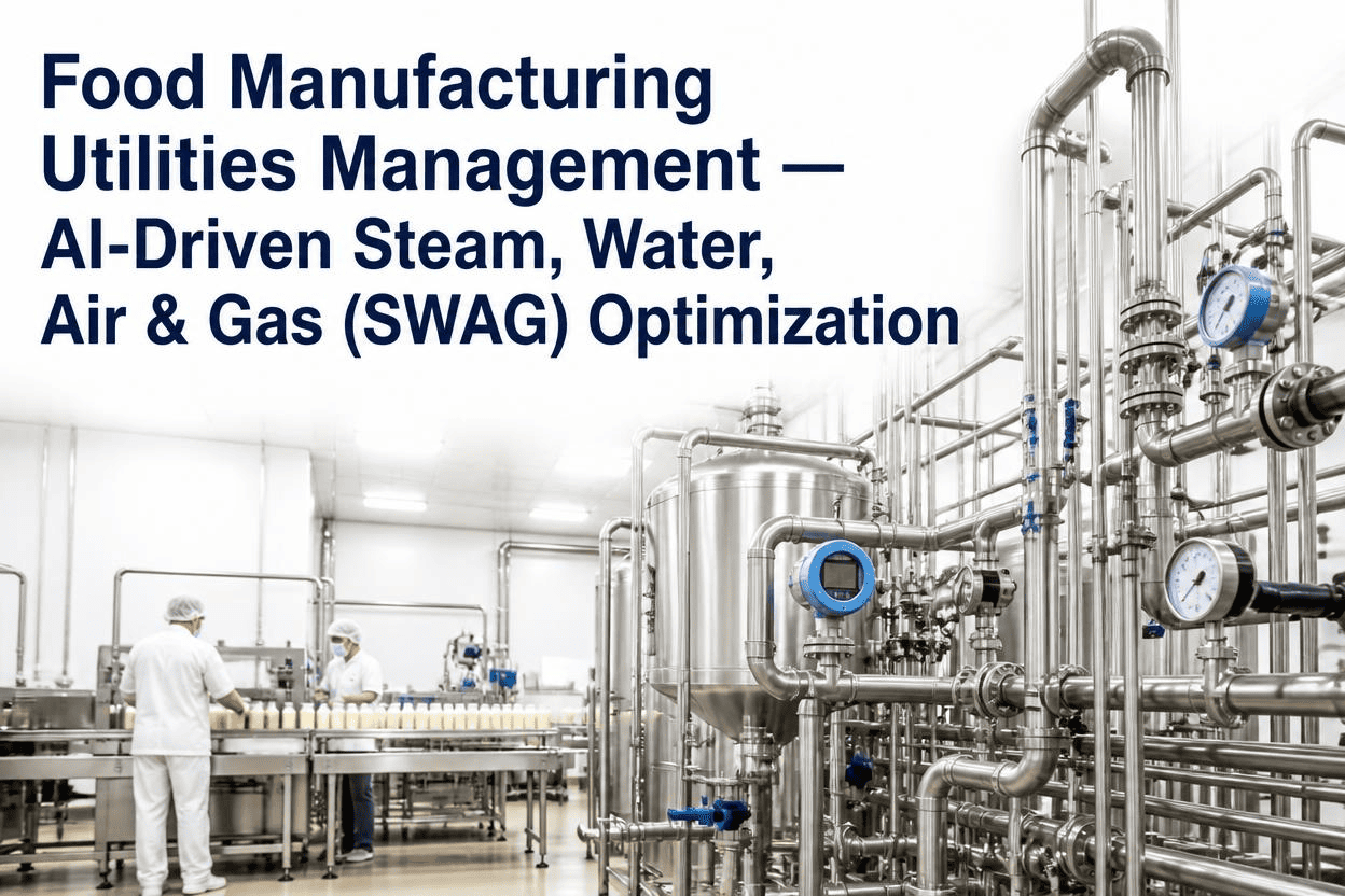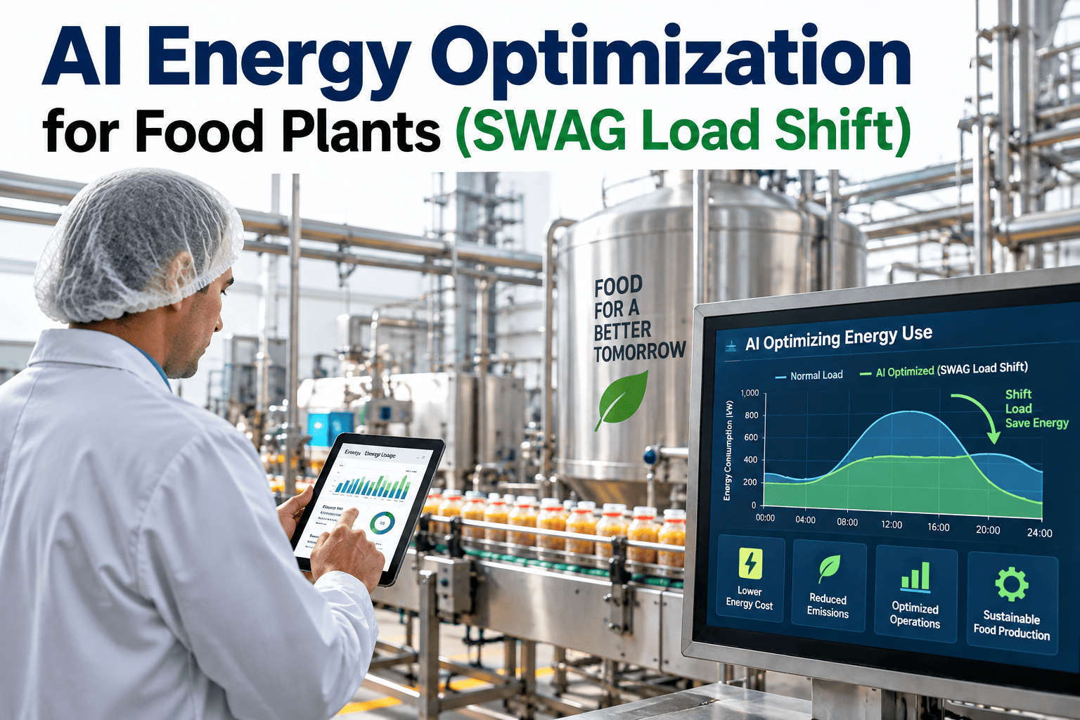
Steam, water, air, and gas — the SWAG utilities — typically account for 25 to 35 percent of total plant operating cost in food and beverage manufacturing, and most of that spend is scheduled by habit rather than by price. Refrigeration compressors cycle on fixed setpoints regardless of the grid's real-time rate, air compressors idle through lunch breaks nobody flags, and steam boilers ramp for a batch that starts twenty minutes late. AI-driven load shifting closes that gap by predicting demand and shifting flexible loads into cheaper, lower-carbon windows. You can walk through your own utility bill against this model with our energy engineering team.
Cut SWAG utility spend without touching production output
iFactory AI predicts refrigeration, compressed air, steam, and water demand hours ahead, then shifts flexible load into your cheapest and cleanest grid windows — automatically, without operator intervention.
Why food plants overpay for utilities they already own
Most food and beverage sites pay time-of-use or demand-charge utility rates, meaning the same kilowatt-hour can cost three to five times more depending on when it is drawn. Fixed operating schedules ignore that entirely, so plants pay peak rates for loads that could just as easily run an hour earlier or later.
A single 15-minute peak sets the demand charge for the entire billing month in most utility tariffs. One compressor bank starting simultaneously with a shift-change refrigeration surge can add thousands of dollars to a monthly bill.
Peak-period electricity commonly runs two to four times the off-peak rate. Refrigeration, water treatment, and CIP heating are all flexible enough to shift, yet most plants run them on a fixed clock regardless of price.
Compressed air leaks, refrigeration short-cycling, and equipment left energized during breaks and changeovers routinely account for 10 to 20 percent of a plant's total utility spend with zero production benefit.
Boilers held at standby pressure for batches that start late burn fuel producing steam nobody uses. Poor coordination between batch scheduling and utility ramp time is one of the largest avoidable gas costs in the plant.
AI demand forecasting for each SWAG utility
iFactory AI builds a separate forecasting model for each utility stream, trained on your production schedule, historical consumption, ambient conditions, and the utility's own rate structure. The models run 6 to 24 hours ahead so shifts can be planned, not reacted to.
Refrigeration and cold storage demand
Compressor load is predicted from ambient temperature, door-open frequency, product loading schedule, and defrost cycle timing. The model pre-cools cold rooms during cheap-rate windows so compressors can throttle back during expensive peak hours without any temperature excursion.
Compressed air demand
Air demand is forecast from the production schedule and historical per-line consumption. Idle compressors are identified during scheduled breaks, changeovers, and low-demand shifts, and staging logic brings only the minimum required compressor bank online.
Steam and boiler load
Boiler ramp timing is synchronized to the actual batch schedule pulled from MES rather than a fixed daily curve, so standby pressure is not held longer than the process requires. Multi-boiler plants get load-balancing recommendations that favor the most efficient unit at part load.
Water and wastewater treatment
RO systems, water heaters, and effluent treatment pumps are flexible loads that can often run overnight. The model schedules these around tank capacity constraints and off-peak electricity windows without affecting production water availability.
What a 24-hour shifted schedule looks like on a real plant
The timeline below shows a simplified refrigeration and compressed air load-shift plan for a mid-size dairy processing plant, mapped against a typical time-of-use rate structure.
The shift is invisible to production. Cold storage temperature never leaves its tolerance band, and compressed air header pressure is held within its normal operating range throughout the entire cycle.
Want to see this modeled against your own rate structure?
Send your utility tariff and a week of interval data. We will show a projected load-shift plan for your refrigeration and compressed air systems before you commit to anything.
Finding phantom loads that never show up on a walkthrough
Phantom load is energy consumed with no corresponding production value — equipment left running through breaks, compressed air leaking behind a wall, or refrigeration short-cycling because a door seal has failed. None of it is visible on a manual walkthrough, but all of it shows up in the interval data.
Weekend and off-shift baseload
Consumption that never drops to true idle during planned downtime usually means equipment is left energized unnecessarily. iFactory flags any asset whose off-shift baseline exceeds its expected standby draw.
Compressed air leak signature
A slow, steady pressure decay during non-production hours with no corresponding demand is the classic leak fingerprint. The model estimates leak volume in real units and ranks leaks by annual cost.
Refrigeration short-cycling
Compressors that start and stop far more frequently than the load requires waste energy on repeated startup current and accelerate mechanical wear. This pattern is usually traced to a failing door seal, defrost timer, or setpoint deadband error.
Simultaneous peak stacking
Multiple large loads starting in the same 15-minute window compound the demand charge even when total daily energy use is unchanged. The model recommends staggered start sequencing to flatten the peak.
Typical results across food and beverage energy AI deployments
The figures below reflect ranges observed across plants that implemented AI-driven load shifting and phantom-load remediation on refrigeration, compressed air, and steam systems.
Fixed schedule versus AI-shifted schedule on a sample tariff
The table below illustrates the cost difference for the same daily energy consumption under a typical time-of-use commercial and industrial rate structure, comparing a fixed operating schedule against an AI-optimized shift plan.
| Rate window | Typical rate multiplier | Fixed schedule draw | AI-shifted schedule draw |
|---|---|---|---|
| Off-peak (12am–6am) | 1.0x baseline | Low — mostly idle equipment | High — pre-cooling, RO, deferred air load released here |
| Mid-peak (6am–10am, 6pm–12am) | 1.5x baseline | Moderate — normal production draw | Moderate — unchanged, no shift needed |
| On-peak (10am–6pm) | 2.5–4x baseline | High — full refrigeration and air load | Reduced — refrigeration coasting on stored cold, minimum air staging |
| Monthly demand charge basis | Set by single 15-min peak | Peak often coincides with shift-change surge | Peak flattened through staggered equipment starts |
How the energy AI layer is deployed without disrupting production
Energy optimization is deployed as a supervisory layer on top of existing refrigeration, compressed air, and boiler controls — not a replacement for them. Every recommendation respects existing safety interlocks and process tolerance bands.
Meter and interval data ingestion
Utility meters, submeters, and existing BMS or SCADA points are connected to build a baseline consumption profile for each utility stream, typically using 4 to 8 weeks of historical interval data.
Rate structure and constraint mapping
Your actual utility tariff, demand-charge structure, and any time-of-use windows are loaded alongside hard constraints — minimum cold storage temperature, minimum air header pressure, and any regulatory hold times.
Shadow mode validation
The model runs in shadow mode, generating shift recommendations without actually controlling equipment, so your engineering team can validate every recommendation against real operating conditions before automation is enabled.
Supervised automation rollout
Once validated, the model is given write access to non-critical setpoints first — typically compressed air staging — and expands to refrigeration and boiler scheduling as confidence builds, always within the tolerance bands set in step two.
FAQ: AI energy optimization for food plants
See what AI load shifting would save on your own utility bill
Bring your last twelve months of utility bills and your rate schedule. We will model where load shifting, phantom-load elimination, and demand-charge flattening apply to your specific plant.