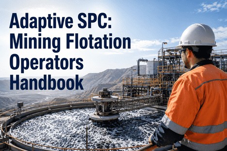
Adaptive SPC Operators: Mining Ore Processing 2026 Guide

By Grace on June 5, 2026

adaptive-spc-limits-mining-ore-processing-operators-defect-elimination

It is 2:17 a.m. on a Wednesday. The flotation circuit operator watches the concentrate grade trend crawl toward the lower spec limit for the third consecutive hour. The SPC dashboard shows green control limits on every parameter. Feed grade, reagent flow, pH, air addition, pulp density, mill power draw. All within the static UCL and LCL that were calculated during last quarter's process capability study. The operator knows something is wrong, but the control chart says everything is fine. By shift handover, the lab confirms the concentrate is off-spec. Eight hours of production tagged for reprocessing. The static control limits that were supposed to protect quality became the reason the defect was missed. This is the cost of fixed SPC limits in a process where ore variability, reagent effectiveness, and equipment response change every shift.

Every Shift Generates the Data for Adaptive Limits. The Question Is Whether Your SPC System Is Using It.
iFactory replaces static control limits with self-tuning limits that continuously recalculate from your process data, catching drift before it becomes a confirmed defect and generating audit-ready documentation without manual chart review.
Why Static UCL and LCL Fail in Ore Processing
Static SPC Limits
Calculated Once, Trusted Forever

  • Limits set from a 30-sample capability study at die tryout or circuit commissioning
  • UCL and LCL remain unchanged until the next manual recalculation, typically quarterly or annually
  • Ore feed hardness shifts, reagent effectiveness drifts with pulp chemistry, mill liners wear, but control limits stay fixed
  • Result: the process leaves the control band, but the SPC chart signals green until the defect is confirmed by lab assay
Misses 60-70% of drift events before they become defects
VS
Adaptive SPC Limits
Self-Tuning with Every New Measurement

  • Control limits recalculated continuously using a rolling window of recent process data (default 100-200 samples)
  • UCL and LCL adapt to real-time changes in feed mineralogy, grind size distribution, reagent response, and environmental conditions
  • The model distinguishes common-cause variation from assignable-cause drift, so operators investigate only real signals
  • Result: limits reflect what the process is doing right now, not what it was doing three months ago
72% fewer nuisance alarms, defects caught 4-6 hours earlier
Your Circuit Already Has the Sensors. Now It Needs the Limits That Make Them Useful.
iFactory connects to your existing historians and delivers adaptive SPC limits that reflect current process conditions, not last quarter's capability study, with a working pilot in weeks, not months.
How Adaptive SPC Limits Work for Operators

Adaptive SPC limits do not require operators to be statisticians. The logic is engineered for the control room, not the lab. Here is what happens inside the system, and what the operator sees, in the sequence it actually occurs on shift.

1
Data Ingestion
The system pulls real-time measurements from every available sensor: mill power draw, feed rate, particle size analyser, pulp density, pH probes, reagent flow meters, froth depth sensors, thickener torque, and online grade analysers. Data arrives at 20-second to 1-minute intervals depending on the instrument.
2
Rolling Limit Calculation
For each parameter, the system maintains a rolling window of the most recent 100-200 data points. The mean and standard deviation of this window are recalculated with every new measurement. The UCL and LCL are set at three sigma from the rolling mean, producing control limits that track the process rather than a historical snapshot.
3
Signal Classification
When a measurement falls outside the adaptive limit, the model determines whether the deviation represents common-cause variation within the process's natural capability band or assignable-cause drift requiring intervention. Only assignable-cause events trigger operator alerts. Common-cause excursions within the natural band are recorded but do not generate alarms.
4
R
Operator Alert + Context
The operator receives an alert that includes: which parameter exceeded its adaptive limit, the deviation magnitude, the current and baseline values, the contribution score if multiple variables are involved, and a timestamped data window for verification. The operator investigates with context, not a blank trend screen.
Operators Should Investigate Real Drift, Not False Alarms.
Adaptive SPC limits cut nuisance alarms by 72% while catching drift events 4 to 6 hours earlier than static control charts, giving operators time to correct before off-spec material is produced.
Adaptive SPC Across the Ore Processing Flow

Each ore processing circuit has distinct dynamics. The parameters that drift in a grinding circuit are different from those in flotation or thickening, and the adaptive limit model must be circuit-specific to capture the correct interaction effects. The table below maps the adaptive SPC approach for each major circuit stage.

Crushing and Grinding
Feed rateMill power draw trendP80 particle sizeCirculating loadPulp densityBall charge level
Adaptive limit priorityMill power running sigma tightens as liners wear, preventing overload events before torque limits are reached
Typical detection lead time2 to 6 hours before P80 exceeds spec
Flotation Recovery
Reagent dosing ratepH trendAir flow per cellFroth depthFeed gradeParticle size
Adaptive limit priorityMultivariate interaction model adjusts reagent UCL/LCL in response to feed grade shifts, preventing both underdosing and overdosing
Typical detection lead time1 to 4 hours before concentrate grade deviation
Thickening and Filtration
Underflow densityFlocculant dosingBed levelFeed solidsThickener torqueFiltrate clarity
Adaptive limit priorityTorque and underflow density limits adjust to changing feed solids, preventing bed collapses and rag layer events
Typical detection lead time2 to 5 hours before moisture spec breach
%
Assay and Grade Control
Online analyser trendXRF sensor readingsSampler intervalAssay lagGrade trajectorySpec boundary proximity
Adaptive limit priorityGrade trajectory limits tighten as the operating point approaches the spec boundary, giving operators early warning before the next lab assay confirms an off-spec result
Typical detection lead timeBefore next assay confirms off-spec
Each Circuit Has a Different Drift Signature. Adaptive Limits Respect That.
Circuit-specific rolling window configuration ensures every stage from grinding to grade control has limits tuned to its time constant and parameter set, with detection lead times that give operators room to act.
Implementing Adaptive SPC Limits on Your Shift

The transition from static to adaptive SPC limits does not require a plant-wide automation upgrade. Most ore processing operations already have the sensor infrastructure and data historian capacity required. The implementation sequence follows a structured path that production teams can execute without disrupting ongoing operations.


Phase 1
Data Audit and Sensor Validation
Identify which process parameters are currently logged to the historian, at what frequency, and whether the instruments are calibrated and returning reliable values. A circuit with unreliable sensors cannot support adaptive limits. Typical audit duration: 2 to 4 weeks.


Phase 2
Rolling Window Configuration
For each parameter, configure the rolling window size, sigma multiplier, and update frequency. Standard configuration uses a 100-sample window at three sigma, but these parameters are adjustable per circuit. The system runs in shadow mode, calculating adaptive limits without triggering alerts, so operators can compare static vs adaptive performance side by side.


Phase 3
Operator Training and Limit Validation
Operators review the adaptive limit behaviour across two to four weeks of production data. Validation confirms that adaptive limits do not produce excessive false alarms and that signal classification matches operator observation. Adjustments to window size and sigma are made based on operator feedback before live activation.

Phase 4
Live Activation with Escalation Workflow
Adaptive limits go live with a defined escalation workflow: parameter-level alert to the operator, circuit-level pattern to the shift supervisor, cross-circuit interaction to the metallurgist. The system logs every alert, operator response, and outcome as structured data for compliance and continuous improvement.
Documented Outcomes from Adaptive SPC Deployments
30-70%
Reduction in defect rates within the first 8 weeks of adaptive limit activation across monitored circuits
72%
Fewer nuisance alarms compared to static SPC, restoring operator trust in control chart signals
4-6 hr
Earlier defect detection versus static limits, giving operators time to correct before off-spec material is produced
8-12 wk
Typical timeline from data audit to live adaptive SPC limits on a single ore processing circuit
Static Limits Protect History. Adaptive Limits Protect the Current Shift.

The ore processing operations that consistently meet concentrate grade specifications, maintain recovery targets, and pass IATF 16949, AS9100, and ISO 9001 audits without recurring non-conformances share one characteristic: their SPC limits reflect what the process is doing right now, not what it was doing at commissioning. Static control limits are a snapshot of past capability. Adaptive limits are a real-time map of current process behaviour. The difference is the difference between investigating a defect after it is confirmed and preventing it before the next lab assay.

For the operator on shift, adaptive SPC limits mean fewer false alarms, earlier warning of real drift events, and a control chart that makes sense for the conditions in front of them, not the conditions their predecessor faced three months ago. For the metallurgist, adaptive limits mean process capability data that reflects actual operating conditions rather than historical averages. For the quality manager, adaptive limits mean documented, timestamped evidence of process monitoring that satisfies audit requirements without manual chart review.

The infrastructure is already in place. The sensors are installed, the historian is recording, and the operators are watching the screens. The missing layer is the adaptive logic that turns raw measurement data into control limits that change when the process changes. That layer is available now, and the operations that deploy it are the ones that will consistently stay inside specification while their competitors investigate the same defects shift after shift. Book a Demo to see adaptive SPC limits running on your circuit data, or Get In Touch to start the data audit for your operation.

Frequently Asked Questions

No. Adaptive SPC limits do not widen arbitrarily. The UCL and LCL are recalculated from the actual standard deviation of the rolling window. If the process is stable and centred, the limits may actually tighten because the model has more data to estimate real variation. If the process drifts, the limits follow the drift, but the system flags assignable-cause deviations separately. The Cpk calculation uses the same formula as traditional SPC; the difference is that the limits reflect real-time process conditions rather than a snapshot from months ago. The result is a chart that is more sensitive to real drift and less sensitive to routine process variation. Book a Demo to see adaptive limit behaviour demonstrated on real ore processing data.

Yes. Adaptive SPC maintains separate limit profiles that can be configured for each ore type, feed grade range, and shift combination. The system automatically detects which ore type is being processed and which shift is operating, then applies the appropriate limit set. The day shift operator sees limits calculated from the day shift's process data, and the night shift operator sees limits from the night shift's data. This eliminates the shift-to-shift Cpk reporting variance that plagues static SPC systems and ensures that each operator is working with control limits that reflect their actual operating conditions. Get In Touch to discuss the ore type profile setup for your operation.

Adaptive SPC requires a minimum of 100 data points per parameter to establish the initial rolling window. At typical ore processing data collection rates (one measurement per minute to one per five minutes), this represents 2 to 8 hours of production data. For circuits with longer time constants, such as thickening where changes propagate over hours, a 200-sample window with a wider sampling interval is recommended. No lengthy historical data set is required for activation. The system learns and adjusts as data accumulates. Get In Touch to schedule a data readiness assessment for your circuits.
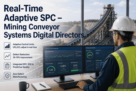
Your Control Limits Are Outdated the Moment the Ore Changes. The Question Is Whether Your SPC System Is Keeping Up.
iFactory's adaptive SPC platform replaces static control limits with self-tuning limits that recalculate from your process data in real time. Operators see limits that reflect current conditions, defects are caught before they are confirmed, and audit-ready documentation is generated automatically without manual chart review or spreadsheet recalculations.

Share This Story, Choose Your Platform!