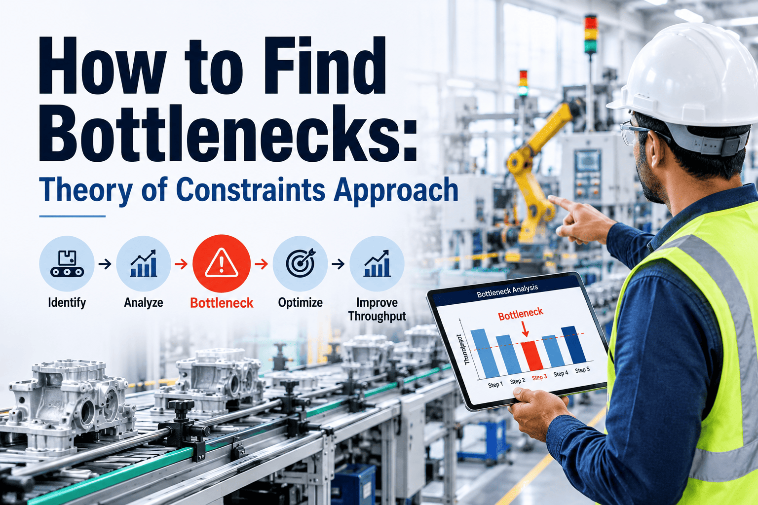
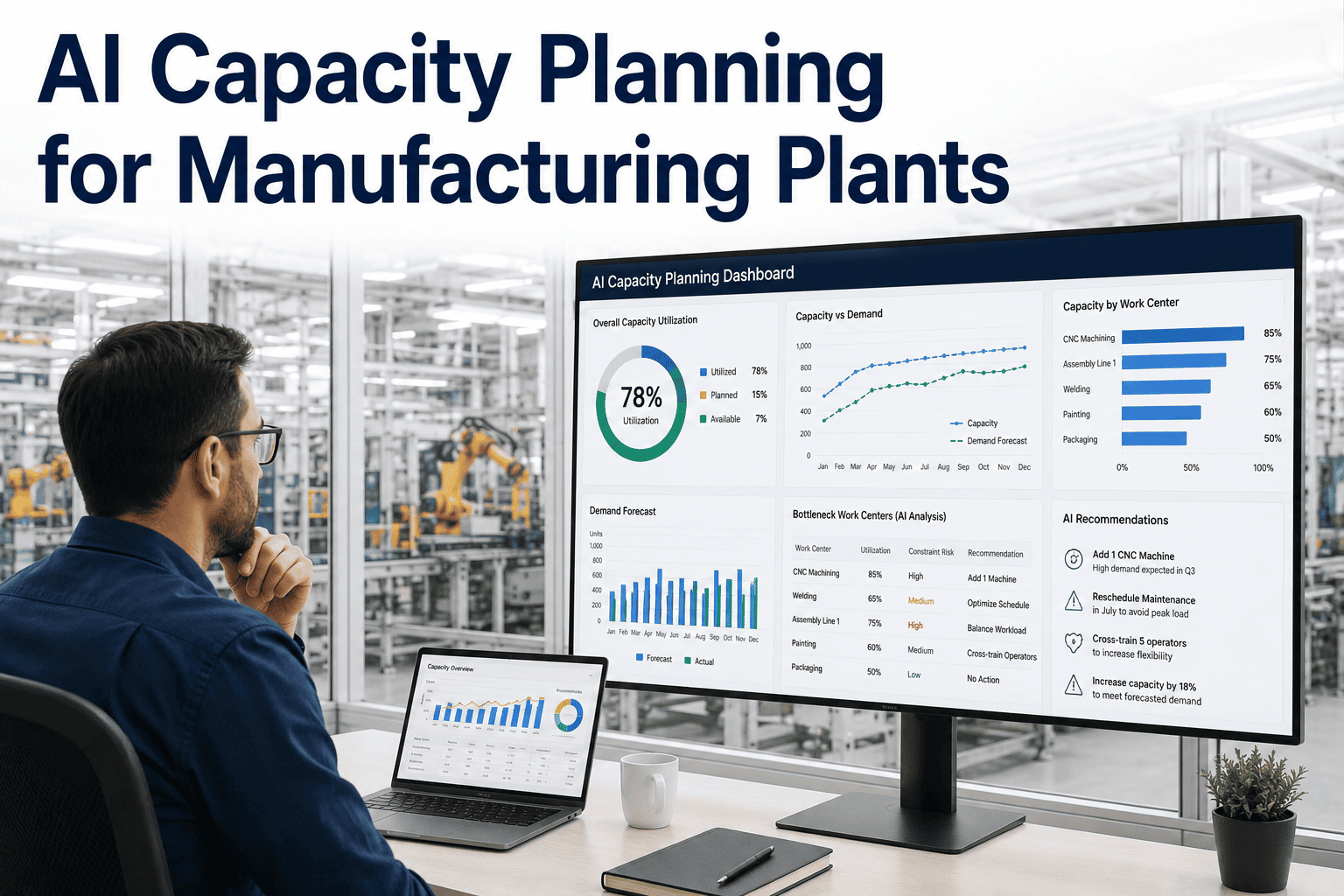
Manufacturing plants lose 15 to 30 percent of potential throughput not because they lack capacity, but because they misidentify where their actual constraint sits. A heat treat furnace that runs at 95 percent utilization gets all the attention, while a finishing station at 78 percent that feeds three packaging lines is the real bottleneck — and nobody notices until shipments start missing. The difference between optimizing the wrong work center and exploiting the true constraint is the difference between a plant that struggles to meet schedule and one that ships on time with headroom. Bottleneck analysis and constraint management are not theoretical exercises — they are the operational lever that determines whether your capacity plan works on paper or works on the floor. Book a demo to see how AI-driven constraint mapping works against your actual production data.
PRODUCTION PLANNING · BOTTLENECK ANALYSIS · CONSTRAINT MANAGEMENT
Most Plants Optimize the Wrong Work Center — Here Is How to Find the Real Constraint
Capacity planning without accurate bottleneck identification is an exercise in moving resources to the wrong place. The busiest machine is rarely the true constraint, and adding capacity to a non-bottleneck work center never increases throughput.
73%
Of Plants Misidentify Their True Bottleneck in Initial Assessments
23%
Average Throughput Recovered After Correct Constraint Identification
8 Weeks
Mean Time to Detect a Shifting Bottleneck Without Continuous Analysis
THE IDENTIFICATION PROBLEM
Apparent Bottlenecks vs. True Constraints — Why Your Busiest Work Center Is Probably Not the Limiting One
The most common mistake in manufacturing capacity planning is equating high utilization with being the bottleneck. Utilization measures how busy a work center is. The bottleneck is the work center that limits the throughput of the entire system. These are not the same thing, and conflating them leads to capacity investments that cost millions and deliver no throughput improvement.
WHAT MOST PLANTS ASSUME
The machine with the longest queue must be the bottleneck
Queues form upstream of bottlenecks, but they also form when upstream work centers batch output inefficiently, when quality problems force rework loops, or when scheduling logic creates artificial waves. A long queue is a symptom, not a diagnosis.
The work center running the most overtime is the constraint
Overtime is often applied to the work center that is easiest to staff for extended hours, not the one that actually limits throughput. A manual finishing operation with flexible labor runs overtime frequently while an automated heat treat furnace at 97 percent utilization with no overtime is the real constraint.
Adding capacity at any highly utilized station will increase output
Adding a shift or a machine at a non-bottleneck work center increases its idle time — it does not increase system throughput. The extra capacity sits unused because the true constraint downstream cannot absorb the additional output. This is the most expensive form of waste in capacity planning.
WHAT CONSTRAINT ANALYSIS ACTUALLY REVEALS
The true constraint is the work center where accumulated wait time exceeds a threshold relative to cycle time across all product routings
Proper bottleneck analysis measures the ratio of wait time to processing time at each work center across every active routing. The constraint is the station where this ratio is highest and most consistent — not the station with the longest absolute queue.
The constraint can shift by product mix, and it does — often within a single planning week
When a plant transitions from Product Family A to Product Family B, the routing changes, the cycle time profile changes, and the constraint often moves to a different work center. Static bottleneck identification assumes a single fixed constraint, which is only accurate in single-product, dedicated-line environments.
Exploiting the constraint — running it continuously with zero idle time — always yields more throughput than adding capacity anywhere else
Theory of Constraints establishes that exploiting the bottleneck is the highest-leverage action. Before any capital is spent on capacity expansion, the constraint should be run with no breaks, no changeover losses, no quality losses, and no starvation. Plants that skip exploitation and jump to elevation routinely overinvest.
CONSTRAINT TAXONOMY
Four Categories of Manufacturing Constraints — And Each One Requires a Different Response
Not all bottlenecks are equipment bottlenecks. A constraint can be a machine, but it can also be a labor skill, a material supply, a policy, or a market condition. Classifying the constraint correctly determines whether the right response is a capital investment, a scheduling change, a training program, or a supplier conversation. Misclassifying the constraint type is the second most common cause of failed capacity planning after misidentifying the constraint location.
01
Physical Capacity Constraints
A machine, furnace, press, or line that cannot produce faster than a certain rate regardless of scheduling, staffing, or input quality. Physical constraints are the most visible and the most frequently over-diagnosed — plants assume a physical constraint when the real limit is a policy or a labor constraint. True physical constraints require either exploitation (maximizing available time) or elevation (adding capital capacity). Before elevating, verify that the machine is actually the system constraint by confirming that no other work center is starving for its output and that wait time ratios confirm it as the limiting node.
Response: Exploit first, then elevate if throughput gain justifies capital
02
Labor and Skill Constraints
A work center limited not by machine speed but by the availability of qualified operators. Common in welding, inspection, CNC setup, and any operation requiring certified skills. A welding station with two qualified welders running two shifts cannot match the output of an automated welding cell, but the constraint is the certified labor pool, not the welding equipment. Labor constraints are often invisible in capacity models that only account for machine hours. They surface as unexplained throughput gaps — the model says the line can produce 40 units per shift but consistently produces 32 because the second welder is pulled for rework or the setup technician is shared across three lines.
Response: Cross-training, certification pipelines, or dedicated crew assignment
03
Material and Supply Constraints
A work center that is capacity-adequate but cannot run because incoming material is late, out of spec, or rationed by a supplier allocation. Material constraints masquerade as capacity problems because the symptom is the same — the work center is not producing — but the root cause is upstream in the supply chain. Plants that respond to a material constraint by adding production capacity waste capital. The correct response is safety stock adjustment, supplier development, dual sourcing, or lead time renegotiation. Material constraints are particularly insidious because they can be intermittent — the supply is adequate for three weeks, then a single delayed shipment creates a constraint that shifts the bottleneck temporarily.
Response: Supply chain restructuring, safety stock, or supplier diversification
04
Policy and Behavioral Constraints
A constraint created not by physical limitation but by a rule, batch size, scheduling policy, or organizational behavior that artificially limits throughput. Common examples: batch sizes set for machine utilization rather than flow, changeover policies that prevent small-lot production, quality hold policies that keep material in quarantine longer than necessary, and scheduling rules that sequence by due date rather than by constraint feeding. Policy constraints are the most difficult to identify because the rule feels correct in isolation — large batches reduce per-unit changeover cost — but creates a system-level bottleneck by creating massive WIP waves that starve downstream work centers between batches.
Response: Policy redesign, batch size optimization, or scheduling logic change
UTILIZATION SPECTRUM
The Capacity Utilization Spectrum — Five Zones That Tell You Whether Your Plant Is Healthy or Heading for a Crisis
Capacity utilization is not a single number to optimize — it is a spectrum with distinct operational characteristics in each zone. Running a plant at the highest possible utilization sounds efficient, but the relationship between utilization and performance is not linear. Beyond the optimal zone, each additional percentage point of utilization increases queue times, reduces flexibility, and raises the probability of missed deliveries at an accelerating rate. The five zones below define what each utilization range actually means for your operation.
The plant has significant idle capacity. Unit costs are high because fixed costs are spread over fewer units. Work centers wait for jobs rather than jobs waiting for work centers. This zone is appropriate during market downturns, product launch ramp-up, or when deliberate capacity buffer is maintained for highly variable demand. The risk is not operational failure — it is financial: the plant is carrying capacity cost it is not using, and the business case for that capacity is eroding each month it sits idle.
The utilization range where throughput, flexibility, and cost are best balanced. Work centers have enough buffer to absorb minor disruptions — a quality hold, a late material delivery, an unplanned absence — without missing shipments. Changeovers can be scheduled without squeezing the available production window. This is the target zone for most mixed-model manufacturing plants. Plants in this zone can respond to demand surges of 15 to 25 percent through overtime and scheduling adjustments without capital investment, which is the definition of a healthy capacity position.
Buffer is thin. Queue times begin to increase non-linearly — a 5 percent increase in load can double wait time at the constraint. Changeover scheduling becomes a weekly negotiation rather than a routine decision. The plant can still hit its schedule under normal conditions, but any disruption — a supplier delay, a quality issue, an equipment failure — cascades into missed deliveries within the same week. Most plants operate in this zone not by design but by drift: demand grows incrementally, capacity is not added, and the plant slowly migrates from optimal into warning without a clear decision point marking the transition.
No meaningful buffer exists. The constraint work center is effectively a single point of failure for the entire plant — any downtime, no matter how brief, translates directly to missed throughput that cannot be recovered within the planning period. Quality problems increase because operators skip inspection steps to maintain output speed. Maintenance is deferred because stopping for preventive maintenance means missing shipments. The plant is running as fast as it can, but the cost of running at this speed — in expediting, quality escapes, overtime fatigue, and customer dissatisfaction — often exceeds the revenue value of the additional units produced.
The plant has committed to more work than it can produce. This is not a utilization problem — it is a planning integrity problem. Backlog grows faster than output. Expediting becomes the default mode of operation. Customer lead times are missed systematically rather than occasionally. The overloaded zone is unsustainable by definition: something breaks, and it is usually the things that are hardest to measure — operator retention, equipment condition, supplier relationships, and customer trust. Plants entering this zone need immediate demand-side action — order deferral, outsourcing, or customer renegotiation — not supply-side action.
Knowing Your Utilization Zone Is the First Step — Knowing Which Work Center Determines It Is the Step Most Plants Skip
Aggregate plant utilization hides the constraint. A plant at 78 percent overall can have a single work center at 96 percent that is already in the critical zone — and that work center is the one determining whether you ship on time. A constraint mapping session against your actual routings and order book takes one call.
DECISION FRAMEWORK
Overtime, Outsourcing, or Expansion — A Structured Framework for the Three Capacity Decisions Every Plant Faces
When the true constraint is identified and exploited, most plants still face a residual capacity gap. The decision about how to close that gap — overtime, outsourcing, or capital expansion — is one of the highest-value financial decisions in manufacturing operations. Each option has a different cost structure, lead time, risk profile, and reversibility. The framework below structures the decision so it is driven by data rather than urgency.
Cost Structure
Premium labor cost at 1.5x to 2x base rate. No capital outlay. Variable cost that scales directly with hours worked. Hidden costs include fatigue-driven quality degradation, absenteeism increase, and turnover in sustained overtime environments.
Lead Time
Immediate to one week. Overtime can be deployed in the current planning week if the labor pool exists and is willing. Union or contractual constraints may limit weekly overtime hours, and sustained overtime triggers premium tier rates in most labor agreements.
Best Suited For
Short-term demand surges of one to eight weeks. Capacity gaps at labor-constrained work centers where the constraint is operator hours, not machine speed. Seasonal peaks that are predictable and bounded in duration.
Break-Even Rule
Economically justified when the contribution margin on additional units exceeds the overtime premium per unit. Loses justification when sustained beyond 8 to 12 weeks, at which point the fatigue and turnover costs typically exceed the margin contribution.
Cost Structure
Supplier quoted price per unit, typically 15 to 40 percent above internal variable cost. No capital outlay. Fixed transportation and quality management overhead. Intellectual property and lead time risks depending on supplier location and capability maturity.
Lead Time
Two to twelve weeks for initial qualification. One to four weeks for repeat orders after qualification. Lead time is the critical variable — if the outsourced capacity cannot deliver within the customer lead time window, the option is structurally infeasible regardless of cost.
Best Suited For
Medium-term capacity gaps of two to six months. Non-core processes where quality risk is manageable. Situations where internal capacity expansion lead time exceeds the demand window. Product families with stable specifications that do not require frequent engineering changes.
Break-Even Rule
Economically justified when the full cost of outsourcing — unit price, freight, quality management, and lead time risk — is less than the cost of lost orders or the amortized cost of temporary capacity expansion over the gap duration.
Cost Structure
Capital expenditure for equipment, installation, and commissioning. Increased fixed cost base that must be absorbed by additional volume. Ongoing maintenance, energy, and labor cost for the new capacity. Highest total cost but lowest per-unit cost at full utilization.
Lead Time
Three to eighteen months depending on equipment lead time, facility preparation, and commissioning requirements. This is the longest lead time option and the primary reason plants default to overtime or outsourcing — they need capacity now, not in six months.
Best Suited For
Permanent demand increases confirmed by contract or sustained order history. Capacity gaps at physical constraints where exploitation and overtime are already exhausted. Strategic decisions to enter new markets or product families that require dedicated capacity.
Break-Even Rule
Economically justified when the net present value of incremental margin over the equipment life exceeds the capital outlay plus increased fixed cost. The decision should be triggered by sustained demand above the exploitation ceiling for a period exceeding the expansion lead time.
AI-DRIVEN CONSTRAINT DETECTION
How AI Changes Bottleneck Analysis — From Quarterly Assessment to Continuous Constraint Mapping
Traditional bottleneck analysis is a periodic exercise: a team of engineers and planners walks the floor, collects queue time data, maps routings, and identifies the constraint. This process takes two to four weeks, produces a snapshot that is accurate for the product mix running during the assessment period, and becomes outdated the moment the mix changes. AI-driven constraint detection replaces this snapshot with a continuous, data-driven view of where the bottleneck sits at any moment — and where it is likely to move next.
MANUAL BOTTLENECK ANALYSIS
Assessment happens quarterly or semi-annually
Between assessments, the bottleneck may have shifted three or four times as the product mix evolved. The plant is optimizing a constraint that no longer exists while the actual constraint goes unmanaged.
Bottleneck identified at aggregate level, not by product routing
A single bottleneck label is assigned to a work center, but that work center may be the constraint for Product Family A and not for Product Family B. Aggregate analysis misses routing-specific constraints that drive specific delivery failures.
No early warning when the constraint is about to shift
The shift is discovered only after throughput drops and shipments miss, because the analysis is backward-looking. By the time the manual assessment identifies the new bottleneck, the plant has already absorbed the cost of the transition period.
Capacity decisions based on a single point-in-time snapshot
Capital expansion decisions justified by a bottleneck assessment that captured one mix profile may be irrelevant by the time the equipment is installed. The investment is based on a constraint that no longer limits throughput.
AI-DRIVEN CONSTRAINT MAPPING
Constraint position updated continuously from live production data
Every shift, the system recalculates wait-time ratios across all work centers and all active routings. The planner sees the current constraint, the previous constraint, and the trend — whether the bottleneck is stable, migrating, or oscillating between two work centers.
Bottleneck identified per routing, per product family, per shift
The system shows that Work Center 7 is the constraint for Routing A but Work Center 3 is the constraint for Routing B — allowing the planner to sequence orders in a way that balances load across both constraints rather than hammering one.
Early warning when utilization trends predict a constraint shift
The system detects that Work Center 12's wait-time ratio has been climbing for four consecutive weeks and projects it will become the system constraint within two weeks if the current order mix continues — giving the planner time to adjust scheduling or prepare capacity.
Capacity decisions grounded in multi-month constraint history
When expansion is considered, the AI provides a constraint history showing how often each work center has been the bottleneck, for which product families, and for how long — turning a single snapshot into a data-backed investment case.
CAPACITY CALCULATION METHODS
Four Capacity Definitions Compared — Knowing Which One You Are Using Determines Whether Your Plan Is Honest
Capacity planning fails most often not because the analysis is wrong, but because different people in the same plant are using different definitions of capacity without realizing it. The production manager quotes rated capacity. The scheduler uses demonstrated capacity. The finance team models effective capacity. The sales team assumes nameplate capacity. Until these definitions are aligned, every capacity conversation is a negotiation between incompatible numbers.
| Capacity Type |
How It Is Calculated |
What It Represents |
Typical Gap from Rated |
When to Use It |
| Rated Capacity |
Available hours multiplied by nameplate production rate |
Theoretical maximum if the work center runs continuously at designed speed with zero losses |
Baseline — 0% |
Equipment specification and capital justification. Never use for scheduling. |
| Effective Capacity |
Rated capacity minus planned downtime, changeovers, and scheduled maintenance |
Realistic maximum output accounting for known non-productive time |
15% — 25% below rated |
Medium-term planning and rough-cut capacity checks. Still optimistic for weekly scheduling. |
| Demonstrated Capacity |
Actual output averaged over the last 8 to 12 weeks of production history |
What the work center has actually produced, including all unplanned losses |
25% — 40% below rated |
Short-term scheduling and load balancing. The most honest number for operational planning. |
| AI-Predicted Capacity |
Demonstrated capacity adjusted by ML model using upcoming mix, maintenance schedule, and constraint position |
Forward-looking capacity estimate that accounts for the specific conditions of the coming period |
Varies — model-dependent |
Detailed scheduling, order promising, and constraint management. Most accurate but requires data infrastructure. |
FREQUENTLY ASKED QUESTIONS
What Production Planning Teams Ask Before Implementing Systematic Bottleneck Analysis
How do you identify the true bottleneck when multiple work centers appear to be running at their limit simultaneously?
When multiple work centers appear constrained, the diagnostic is to measure the cumulative wait time at each station relative to its processing time across all active routings over a representative period — typically four to eight weeks. The true system constraint is the single work center where this ratio is highest and most consistent. Apparent constraints at other stations are almost always caused by the upstream effect of the true bottleneck: when the constraint is slow, it starves downstream stations and backs up upstream stations, making multiple areas look constrained simultaneously. Resolving the true bottleneck relieves pressure at the apparent constraints without any action at those stations.
Book a demo to see this analysis run against your production data.
What is the difference between capacity utilization and OEE, and which metric should drive capacity planning decisions?
OEE measures how effectively a work center uses its planned production time — it multiplies availability, performance, and quality to produce a single percentage. Capacity utilization measures how much of the total available time — including planned downtime — is used for production. They answer different questions: OEE tells you whether the work center is performing well during the time it is scheduled to run. Capacity utilization tells you whether you are using enough of the total available capacity to justify the fixed cost of that capacity. For capacity planning, utilization is the primary metric because it drives the expansion, overtime, and outsourcing decisions. OEE is the primary metric for operational improvement within the existing capacity envelope.
Talk to our support team about setting up the right measurement framework for your plant.
How often should we reassess where the bottleneck is, and what triggers a re-assessment?
In a plant with a stable, single-product dedicated line, the bottleneck rarely moves and a quarterly check is sufficient. In a mixed-model plant with more than three product families and variable order mix, the bottleneck can shift with each major scheduling change — meaning the constraint position should be evaluated weekly at minimum. The specific triggers for an immediate re-assessment include any significant change in product mix share, the introduction of a new product family, the loss of a major customer or addition of a new one, a change in supplier lead times that affects material availability, and any equipment change that alters cycle times on a routing. AI-driven constraint detection eliminates this question by making re-assessment continuous rather than event-triggered.
Book a demo to see continuous constraint mapping in action.
We added a machine to what we thought was the bottleneck and throughput did not increase. What went wrong?
This is the most common outcome of misidentified bottleneck analysis. When capacity is added at a non-constraint work center, the new capacity sits idle because the true bottleneck downstream cannot absorb the additional output. The non-constraint was busy but not limiting — it was a symptom of the real constraint, not the cause. The correct response is not to add more capacity elsewhere but to identify the actual constraint using wait-time ratio analysis across all routings. In many cases, the original machine addition was not wasted — it provides buffer that will be useful once the true constraint is elevated — but the throughput gain will not materialize until the true limiting work center is addressed.
Contact support for a diagnostic review of your capacity investment and constraint position.
How does AI-driven capacity planning integrate with our existing ERP and MES systems?
AI capacity planning does not replace your ERP or MES — it reads from them. The integration path pulls production order data, work center status, routing definitions, actual cycle times, and shift logs from the MES and ERP through standard read APIs or database connections. The AI layer calculates constraint positions, utilization trends, and capacity forecasts using this data and presents the results through a planning interface or pushes them back into the ERP as adjusted capacity figures for the planning run. No write access to control systems is required, and no changes to existing ERP or MES configurations are needed. The deployment is a read-only integration that adds analytical capability without disrupting current workflows.
Book a demo to see the integration architecture mapped to your systems.
MAP YOUR CONSTRAINTS
Your Plant Has a Bottleneck — the Question Is Whether You Are Managing It or It Is Managing You
A constraint mapping session against your actual production routings, order history, and work center data takes one call. You will see where the bottleneck sits today, where it has been for the last quarter, and where it is likely to move next — with a clear recommendation for the highest-leverage action.