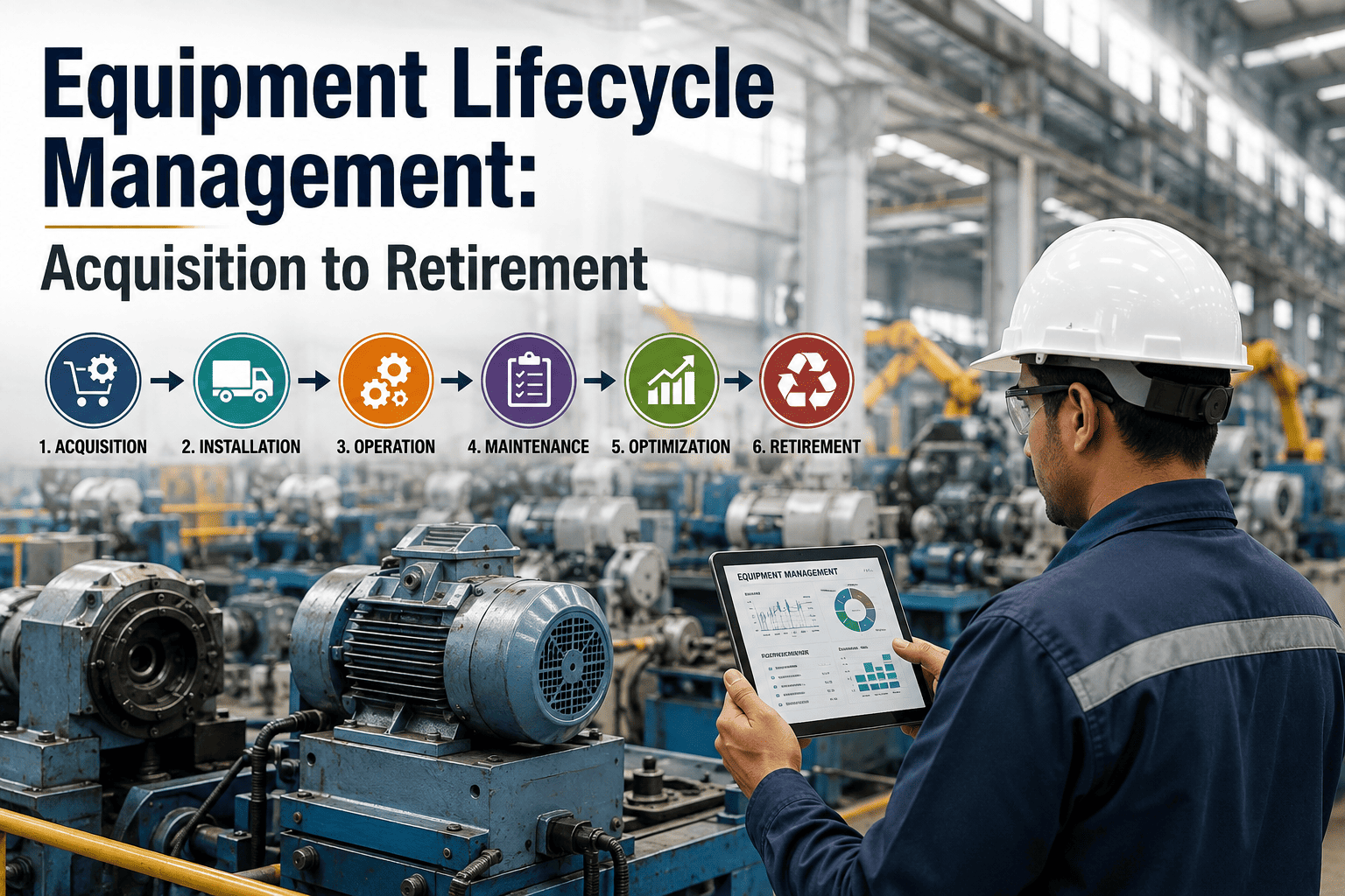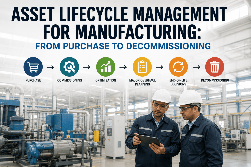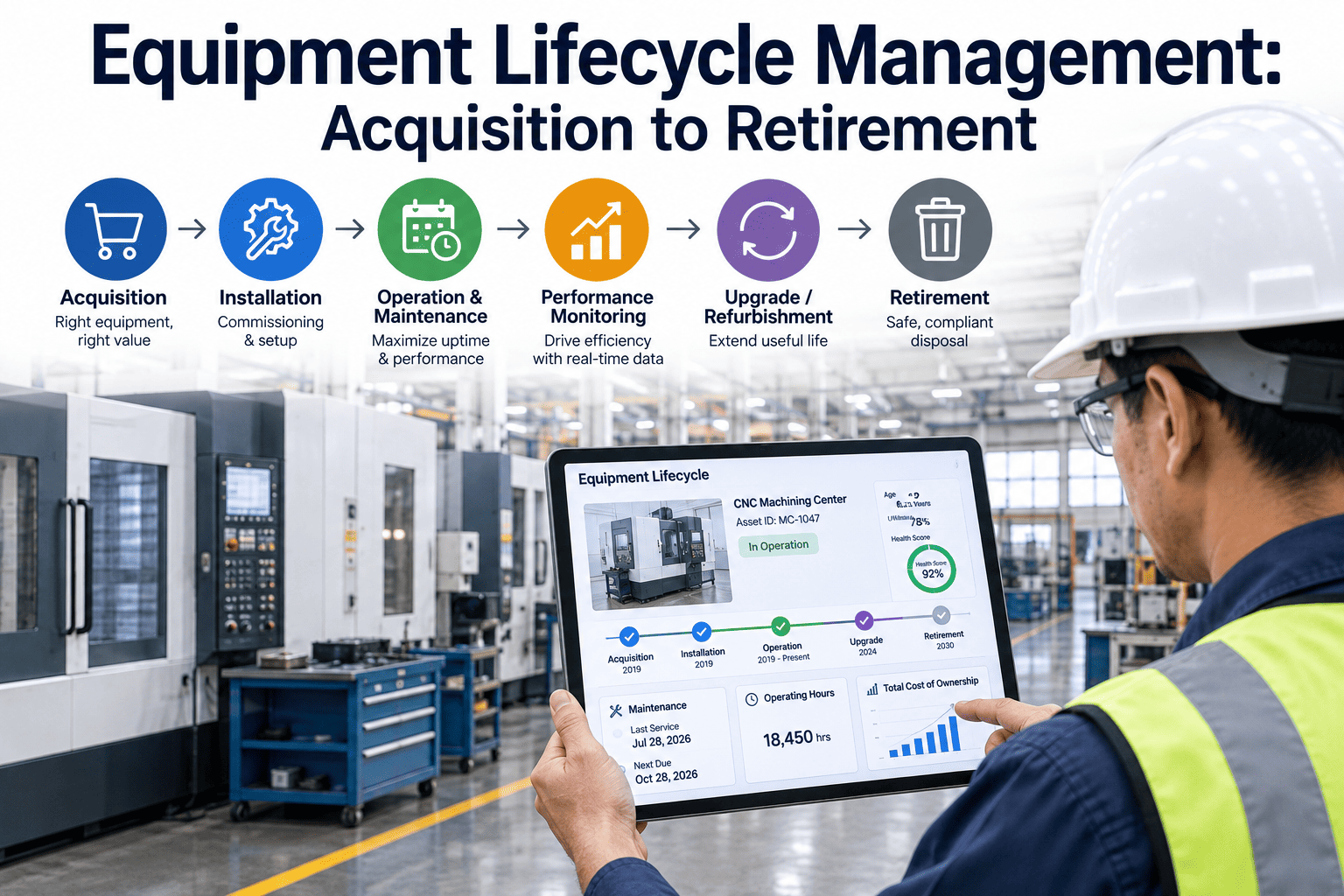
The invoice for a new machine is the smallest number you will ever attach to that asset. Purchase price accounts for only 18-25% of what a production asset actually costs before it leaves your floor for the last time — the rest arrives quietly as energy draw, spare parts, technician hours, unplanned stoppages and a decommissioning bill nobody budgeted for. Equipment lifecycle management is the discipline of controlling every one of those dollars from specification through retirement. See how iFactory turns that scattered history into one connected asset record for every machine you own.
From Purchase Order to Scrap Value — Manage the Whole Life of Every Machine
The Cost You Approved Versus the Cost You Actually Signed Up For
Capital approval processes are built around a single visible number: the quoted price of the equipment. Everything that follows — the electricity it draws for the next fifteen years, the bearing kits, the technician overtime on a Sunday night, the production hours lost when it stops mid-shift, the rigging crew that eventually removes it — lands in different budgets, owned by different managers, reported in different systems. Nobody adds them together, so nobody sees that the machine that looked cheapest at bid stage became the most expensive asset in the plant by year six. Industry benchmarks consistently put acquisition at roughly a fifth to two-fifths of lifetime spend, with the balance accumulating across operation, maintenance and end-of-life handling.
The practical consequence is a plant full of assets whose true performance nobody can defend with numbers. Finance depreciates on a fixed schedule that has no relationship to actual condition. Maintenance carries assets that have quietly entered wear-out and are consuming the repair budget of three healthy machines. Procurement re-orders the same model that has been the worst performer on the floor, because the reorder was priced, not evaluated. Lifecycle management fixes the visibility problem first — everything else follows from having the full cost picture attached to the asset itself rather than scattered across five systems that never talk.
The Six Stages Every Asset Passes Through
Lifecycle management is not a maintenance activity with a wider scope. It is a sequence of six decision points, each owned by a different function, each capable of destroying value created by the stage before it. A specification written without maintenance input produces a machine nobody on your floor can service. A commissioning handover done on paper produces an asset with no baseline, so five years later nobody can tell whether current vibration readings are normal or alarming. A retirement decision made without cost history produces either a premature write-off of a healthy machine or a two-year overrun on a machine that should have been replaced.
The value of running these six stages on one platform is continuity of evidence. The specification survives into procurement as a scoring sheet. Procurement scores survive into commissioning as the acceptance criteria. Commissioning baselines survive into operation as the reference for condition monitoring. Operating history survives into the replacement business case as proof. Nothing has to be reconstructed from memory, and no stage begins with somebody hunting through an inbox for a PDF that may or may not still exist.
Below is what each stage owns in practice, the cost lever it controls, and the failure mode that shows up when the stage is run without data. The table scrolls sideways on smaller screens so the full comparison stays intact rather than collapsing into fragments.
| Lifecycle stage | Primary owner | Cost lever controlled | Typical failure without data | What the record must hold |
|---|---|---|---|---|
| Specification | Engineering and reliability | Sets 60-80% of future maintainability | Machine specified for peak output nobody ever runs, at permanent energy penalty | Duty profile, service access, parts lead time, target lifecycle cost |
| Procurement | Purchasing and finance | Locks capital, warranty and parts pricing | Lowest bid selected, 40-60% higher lifetime cost accepted unknowingly | TCO score sheet, service terms, consumable pricing, uptime guarantees |
| Installation and commissioning | Projects and maintenance | Determines infant mortality rate | No baseline captured, so early drift is invisible for the first two years | Serials, drawings, PM schedule, warranty dates, baseline readings |
| Operation | Production | Drives 25-30% energy and labour share | Overloading and setup abuse recorded nowhere, blamed on the machine later | Runtime hours, output rate, energy per unit, operator and shift tagging |
| Maintenance | Maintenance and reliability | Drives 30-45% of lifetime spend | Calendar PM applied uniformly, over-serving healthy assets and under-serving worn ones | Work orders, parts consumed, labour hours, failure codes, MTBF trend |
| Retirement and disposal | Finance and operations | Recovers or forfeits residual value | Emergency replacement at premium price with no salvage recovery | Cumulative cost, condition score, resale value, compliance certificates |
Reading Where an Asset Sits on Its Failure Curve
Most physical assets follow the same failure pattern across their life: a spike of early failures caused by installation defects and commissioning errors, a long stable middle where failures are random and rare, and a rising tail as wear-out sets in. The mistake plants make is applying one maintenance strategy across all three phases. Preventive intervals that are correct in year four are wasteful in year two and dangerously loose in year eleven. Knowing which phase an asset occupies is what converts a maintenance budget from a flat cost into a targeted investment, because effort moves toward the assets that are actually degrading.
Mean time between failures, tracked over successive periods, is the clearest indicator of position on the curve. A reliability signal that has declined across three or more consecutive periods while preventive compliance stayed above ninety percent is the accepted trigger to begin replacement planning — not a single dramatic breakdown, and not the asset's age on the depreciation schedule. That distinction alone prevents both categories of expensive error: scrapping healthy machines and nursing exhausted ones.
Find Out Which of Your Machines Have Already Crossed Into Wear-Out
The Repair or Replace Decision, Scored Instead of Argued
Repair or replace is the most expensive recurring decision in plant operations, and it is usually settled in a meeting by whoever argues most confidently. Replace too early and capital is spent on machines with years of productive life remaining. Replace too late and the operation absorbs escalating repair bills, quality drift, safety exposure and the premium cost of buying under duress. In 2026 the arithmetic has tightened further, because replacement equipment carries longer lead times and elevated pricing, which makes a documented, condition-based case more valuable than it has ever been.
A scored framework removes the argument. Each criterion carries a weight, each asset gets a number, and the threshold for action is agreed before any specific machine is on the table. The scorecard below is the structure iFactory applies against live maintenance history, and because the inputs are already captured in the lifecycle record, the score updates itself every month rather than being assembled by hand for a budget meeting.
| Decision criterion | Weight | Repair is indicated when | Replace is indicated when | Data source in the lifecycle record |
|---|---|---|---|---|
| Annual corrective cost against replacement value | High | Below 25% of current replacement value | Sustained at 40-60% or higher | Work order cost roll-up per asset |
| Reliability trend | High | Stable or improving across periods | Declining across three consecutive periods | Mean time between failures history |
| Remaining useful life | High | Three or more productive years supported by condition data | Under eighteen months with accelerating wear | Condition monitoring and degradation model |
| Downtime impact on production | High | Asset has redundancy or slack capacity | Single point of failure on a constrained line | Criticality rating and stoppage log |
| Spare parts availability | Medium | Parts stocked and supported by the manufacturer | Obsolete components, long lead times, grey market sourcing | Parts catalogue and supplier status flag |
| Energy and yield performance | Medium | Within ten percent of design specification | Sustained energy or scrap penalty versus current technology | Energy per unit and quality yield trend |
| Safety and compliance exposure | High | Guarding, controls and certifications current | Non-compliant controls or unresolved incident history | Inspection results and incident records |
| Replacement lead time and install scope | Medium | Repair restores specification within the planned outage | Lead time fits a planned shutdown window ahead | Procurement history and project schedule |
A Worked Example: Why the Cheaper Machine Costs More
The clearest way to see lifecycle economics is to run two realistic options side by side over the same service period. Both machines below do the same job at the same rated output. One costs significantly less to buy. Over ten years the ranking reverses completely, and the gap is not marginal — it is larger than the original purchase price of either unit. This is the pattern behind the repeated industry finding that purchase-price selection routinely locks in forty to sixty percent higher lifetime cost.
The figures below are illustrative and rounded for clarity, using cost categories that any plant can populate from its own records. What matters is not the exact numbers but the structure: once energy, maintenance, downtime and disposal are placed in the same column as capital, the decision becomes obvious and defensible. The same model, populated with your actual utilisation and failure history, is what turns a procurement preference into an approved business case.
| Ten-year cost category | Option A: lower purchase price | Option B: higher specification | Difference over the period |
|---|---|---|---|
| Acquisition, freight and installation | $260,000 | $330,000 | Option B costs $70,000 more up front |
| Energy consumption across ten years | $410,000 | $285,000 | Option B saves $125,000 |
| Preventive maintenance and consumables | $190,000 | $160,000 | Option B saves $30,000 |
| Corrective repair and spare parts | $275,000 | $140,000 | Option B saves $135,000 |
| Unplanned downtime and lost output | $340,000 | $155,000 | Option B saves $185,000 |
| Decommissioning less residual value | $25,000 | $8,000 | Option B saves $17,000 |
| Ten-year total cost of ownership | $1,500,000 | $1,078,000 | Option B is $422,000 cheaper to own |
Five Signals That Retirement Planning Should Already Have Started
Retirement is the stage most operations handle worst, because it is the only one that has no natural trigger. Specification begins when a project is approved, procurement begins when a specification is signed, commissioning begins when the truck arrives — but nothing forces a retirement conversation until the machine fails badly enough to stop the line. By then the decision is being made under pressure, with no time to compare options, negotiate lead times, plan the installation window or recover residual value from the outgoing asset. Planned capital replacement is consistently cheaper than emergency replacement, and the difference is largely a function of how early the conversation started.
The five signals below are the ones that reliably appear twelve to eighteen months before an asset becomes a crisis. Each one is measurable from data a lifecycle platform already holds, which means the warning can be automated rather than depending on someone noticing a pattern across a year of work orders. When two or more of these fire on the same asset, the replacement case should move into the capital planning cycle immediately rather than waiting for the next budget round.
What Retirement Done Properly Actually Recovers
Decommissioning is treated as an expense line, but a planned retirement recovers value in four directions at once. There is the residual value of the asset itself, which collapses to near zero once a machine has been run to catastrophic failure but holds meaningfully when it is retired in working order. There is the spare parts inventory tied to that asset, which can be liquidated or redeployed instead of quietly written off two years later. There is the floor space and the connected utility capacity, which have real value in any plant running near its footprint limit. And there is the operating history itself, which becomes the specification input for the replacement.
Environmental and compliance obligations also close out more cleanly under a planned process. Hazardous fluids, refrigerants, contaminated components and recycling documentation all have handling requirements that are cheaper and safer to satisfy on a scheduled basis than during an emergency removal. Keeping those certificates attached to the retired asset record closes the audit trail permanently, so that a query three years later has an answer that does not depend on anyone remembering which contractor did the removal.
How iFactory Runs the Full Lifecycle on One Platform
iFactory connects the six lifecycle stages into a single asset record that follows the machine from the first specification document to the disposal certificate. The platform sits across your existing plant systems rather than replacing them, pulling condition and utilisation data from equipment already on the floor, work order history from your maintenance function, and cost data from the systems finance already trusts. What it adds is the connective layer that turns those separate streams into a lifecycle position, a cost curve and a decision trigger for every asset you own.
Deployment is delivered as a turnkey package rather than a software licence and a training manual. The AI compute node arrives pre-configured and racked, ready for power and network, with cabling, network configuration, controller and historian integration, operator training and continuous remote monitoring included in the scope. Typical sites reach live operation in six to twelve weeks across three phases, and the platform runs with 99.9% uptime across a base of more than a thousand industrial clients.
What Changes in the First Twelve Months
The measurable returns from lifecycle management show up in numbers the operation already tracks, which is what makes the business case straightforward to defend. Downtime falls because degradation is caught before it becomes failure. Maintenance cost falls because effort is directed at assets that need it instead of spread evenly across the register. Capital spend becomes predictable because replacement is planned rather than triggered by breakdown. And asset life extends, because the machines that are healthy stop being replaced on an arbitrary schedule.