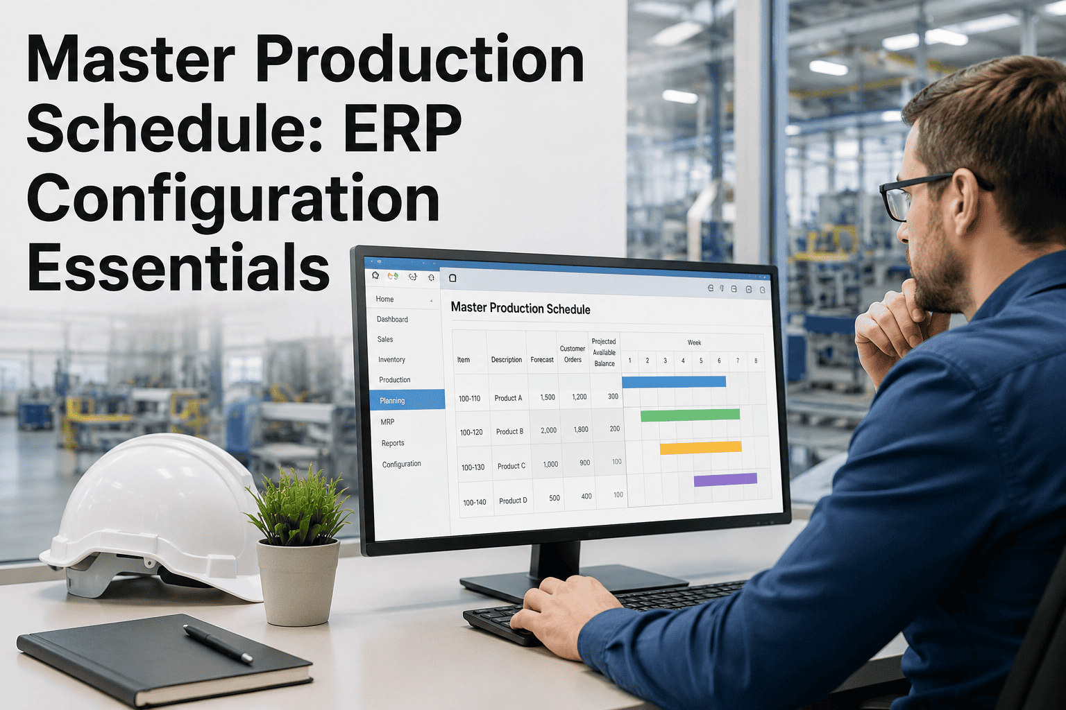
The master production schedule is the single most consequential configuration in any manufacturing ERP, yet most plants set it up during implementation and never revisit the parameters. Planning horizons get defined based on supplier lead times from three years ago. Time fences stay at their default values regardless of whether the actual order volatility has changed. Order promising logic runs on ATP rules that do not reflect the real capacity constraints on the floor. The result is an MPS that generates MRP runs planners do not trust, schedules that change daily, and a planning process that exists on paper but does not drive actual shop floor execution. Fixing the MPS configuration is not a tuning exercise — it is the highest-leverage planning improvement most plants can make without adding any new software. Book a demo to see what a properly configured MPS looks like against your actual order book.
PRODUCTION PLANNING · MPS CONFIGURATION · ERP SETUP
Your Master Production Schedule Is Configured Wrong — and Your Planners Know It
The MPS parameters set during ERP implementation were reasonable guesses. Three years of demand shifts, lead time changes, and mix volatility later, those same parameters are generating schedules your planning team overrides every week.
68%
Of Plants Still Run on Default MPS Parameters Set at Go-Live
3.2x
More Schedule Changes in Plants With Unconfigured Time Fences
41%
Of MRP Exceptions Caused by MPS Instability Rather Than Actual Demand Changes
12 Weeks
Average Time to Stabilize an MPS After Correct Parameter Configuration
THE STABILITY PROBLEM
An Unstable MPS Does Not Just Annoy Planners — It Propagates Errors Through Every downstream System
Schedule instability is the condition where the MPS changes more frequently or more significantly than the actual demand signal justifies. It is not caused by demand volatility alone — it is caused by MPS parameters that allow the schedule to react to noise rather than signal. When the MPS is unstable, every system that depends on it amplifies the instability: MRP generates unnecessary change notices, procurement places expedited orders for shifts that will be rescheduled again next week, and the shop floor learns to ignore the schedule entirely.
Every MPS change triggers a full or partial MRP regeneration. When the MPS for a component changes three times in a week, MRP generates three sets of planned orders, three sets of cancellation messages, and three sets of reschedule-in and reschedule-out notices. Planners spend their mornings processing exceptions that will be obsolete by afternoon. The MRP exception report — which should be the primary planning tool — becomes noise that masks the real action items. Studies across manufacturing ERP deployments consistently show that 35 to 50 percent of MRP exceptions are caused by MPS instability rather than genuine demand or supply changes.
Purchasing receives reschedule notices for raw materials and components that have already been ordered, received, or are in transit. The buyer must evaluate each notice, determine whether the change is real or noise, contact the supplier if the order needs adjustment, and track the revised delivery. For suppliers with long lead times — castings, forgings, specialty chemicals — the reschedule notice arrives after the supplier has already committed capacity. The result is a supplier relationship degraded by constant changes that the supplier correctly identifies as buyer-side planning problems, not genuine demand shifts.
When the production schedule changes daily, supervisors stop using it as an execution tool. They develop their own parallel scheduling methods — whiteboards, spreadsheets, verbal agreements — that are invisible to the ERP and invisible to the planning team. The formal schedule and the actual execution diverge, and the ERP data becomes a fiction that everyone acknowledges but no one fixes. Recovering from this state takes months of stable scheduling behavior, which is impossible until the MPS parameters that caused the instability are corrected.
04
Customer Lead Time Erosion
Order promising uses the MPS to determine available-to-promise quantities and dates. When the MPS is unstable, the ATP picture changes every time the schedule changes — meaning the delivery date quoted to the customer on Monday may not be achievable by Wednesday because the MPS shifted. The sales team loses confidence in the dates the system provides and starts adding informal buffer to every promise, effectively extending quoted lead times beyond what the plant can actually achieve. The customer experiences longer lead times not because the plant is slow, but because the planning system is unstable.
PLANNING HORIZON ARCHITECTURE
The Planning Horizon Is Not One Window — It Is Three Zones With Different Rules in Each
A planning horizon is the total time span the MPS covers — typically 12 to 52 weeks depending on the cumulative lead time of the product. But within that horizon, not all time periods are governed by the same rules. The planning horizon is divided into three distinct zones, each with a different purpose, a different level of schedule stability, and a different set of allowed changes. Misunderstanding these zones is the most common root cause of MPS instability.
NEAR-TERM ZONE
Week 1 Through Week 4
Purpose
Execution driving. This zone contains orders that are released to the shop floor, materials that are on hand or in transit, and capacity that is allocated. Changes in this zone directly disrupt operations.
Stability Requirement
Maximum stability. Schedule changes in this zone should require management approval and should be limited to genuine emergencies — customer cancellations, quality failures, or equipment breakdowns. The target is zero voluntary changes.
Allowed Changes
Quantity decreases within pre-approved tolerances. Order splits if material and capacity exist. Date shifts of one to two days with supervisor confirmation. No quantity increases, no new order insertions, no priority changes without formal override.
8% of total horizon — highest protection
MID-TERM ZONE
Week 5 Through Week 12
Purpose
Planning and procurement driving. This zone contains orders where materials are being procured, capacity is being reserved, and supplier deliveries are being scheduled. Changes here affect procurement but not yet execution.
Stability Requirement
Controlled flexibility. The planner can adjust quantities and dates within defined tolerances without special approval, but changes beyond tolerance thresholds require a formal review. The goal is to absorb demand variation here before it reaches the near-term zone.
Allowed Changes
Quantity adjustments within plus or minus 15 to 20 percent. Date shifts within one week. New order insertions if material availability is confirmed. Product mix swaps within the same product family if routing and capacity impact is assessed.
17% of total horizon — controlled flexibility
LONG-TERM ZONE
Week 13 Through Week 52
Purpose
Demand planning and capacity planning. This zone contains forecast-driven planned orders that exist to signal future material and capacity requirements. The numbers here are planning estimates, not commitments.
Stability Requirement
Full flexibility. The planner and the demand planning team can adjust forecast quantities, shift timing, and reconfigure the product mix freely. The only constraint is that changes should be reflected in the demand forecast rather than as direct MPS overrides to maintain the forecast-to-MPS traceability.
Allowed Changes
Unrestricted forecast adjustments. Product family reconfiguration. Capacity planning scenario analysis. New product introduction scheduling. Long-lead material procurement triggering based on planning thresholds.
75% of total horizon — full flexibility
TIME FENCE CONFIGURATION
Time Fences Are the Enforcement Mechanism — Without Them, Your Planning Zones Are Suggestions, Not Rules
Time fences are the dates within the planning horizon where the rules for schedule changes shift. They are the boundaries between the near-term, mid-term, and long-term zones described above. Every ERP system supports time fences, but most plants either leave them at default values or set them once and forget them. The correct time fence configuration depends on the cumulative lead time, the supplier flexibility, and the actual change tolerance the shop floor can absorb — not on a generic template from the implementation guide.
Frozen Zone
No automatic changes. Manual override required with approval chain.
Set At: Cumulative manufacturing lead time minus one week
Typical Range: Week 1 to Week 3
ERP Setting: Planning time fence — disallow automatic reschedule
Firm Zone
Limited changes allowed within tolerance. Planner discretion for small adjustments.
Set At: Cumulative lead time plus shortest supplier lead time
Typical Range: Week 4 to Week 8
ERP Setting: Demand time fence — allow reschedule within tolerance %
Flexible Zone
Full planner control. System generates suggestions but planner decides.
Set At: Longest procurement lead time for critical materials
Typical Range: Week 9 to Week 16
ERP Setting: Release time fence — planner can accept or reject MPS suggestions
Free Zone
Forecast-driven. System manages automatically based on demand inputs.
Set At: End of planning horizon
Typical Range: Week 17 to Week 52
ERP Setting: Beyond all time fences — fully automated MPS generation
Time Fences Set at Implementation Are Almost Never Right Three Years Later — and Your Planners Are Compensating Manually Every Week
If your planning team is manually overriding the MPS more than twice per week in the frozen zone, the fence configuration is wrong. A structured review of your actual change patterns against your fence settings takes one session and eliminates the majority of manual overrides.
ORDER PROMISING LOGIC
ATP vs. CTP — The Order Promising Decision That Determines Whether You Keep or Lose the Customer
When a customer requests a delivery date, the ERP system must determine whether that date is achievable. The two methods for making this determination — Available-to-Promise and Capable-to-Promise — produce different answers for the same order, and choosing the wrong method either over-promises and misses delivery or under-promises and loses the order to a competitor. Most ERP systems default to ATP because it is simpler to configure, but ATP does not consider capacity constraints — it only checks inventory and planned receipts.
AVAILABLE-TO-PROMISE
What It Checks
On-hand inventory, planned production orders, planned purchase receipts, and allocated quantities. It answers: do we have the stuff, or will we have it by the requested date?
What It Does Not Check
Work center capacity, labor availability, tooling constraints, or the current load on the constraint work center. It assumes that if material is available, capacity is available — which is false at or near the constraint.
When It Works
Plants with significant capacity buffer — utilization below 70 percent — where material availability is the primary order qualifier and capacity is rarely the limiter. Also appropriate for distribution environments where the promise is from warehouse stock rather than production.
When It Fails
Plants running above 80 percent utilization where the constraint work center determines throughput. ATP will promise dates that material availability supports but capacity cannot deliver — resulting in accepted orders that miss their promised date.
Verdict: Use only when capacity is proven not to be a limiting factor
CAPABLE-TO-PROMISE
What It Checks
Everything ATP checks, plus work center capacity, routing times, current shop floor load, constraint position, and available overtime. It answers: can we actually produce and deliver by the requested date?
What It Requires
Accurate routing data, current work center load, a defined constraint position, and a planning horizon long enough to simulate the production path. CTP is more complex to configure because it depends on the quality of the capacity model, not just the inventory model.
When It Works
Plants running above 75 percent utilization, mixed-model environments where different products load different work centers, and any make-to-order environment where the order promise commits actual production capacity rather than warehouse stock.
When It Fails
When the underlying capacity data is inaccurate — wrong routing times, outdated work center rates, or a constraint position that does not reflect reality. A CTP promise based on bad capacity data is worse than an ATP promise because it carries a false sense of precision.
Verdict: Use when capacity is a real or potential order qualifier
ROUGH-CUT CAPACITY PLANNING
RCCP Is the Checkpoint Between the MPS and MRP — Skip It and You Propagate Infeasible Plans
Rough-Cut Capacity Planning evaluates whether the master production schedule is feasible given the capacity of critical work centers — typically the bottleneck and a few near-bottleneck stations. It runs before MRP, which means it catches infeasible schedules before they generate purchase orders and planned production orders that the floor cannot execute. Despite this, many plants either skip RCCP entirely or run it as a post-hoc report that nobody acts on. The RCCP configuration in the ERP determines whether it functions as a genuine planning checkpoint or a checkbox on the implementation timeline.
01
Define Resource Profiles
For each critical work center, define the capacity profile — available hours per shift, number of shifts, planned maintenance windows, and historical efficiency factors. This is not the same as the work center master data in the routing; it is a planning-level approximation that aggregates across product families. The profile should reflect realistic capacity, not theoretical nameplate capacity, and should be reviewed monthly as conditions change.
02
Map Bill of Capacity
For each MPS item or product family, define the capacity consumption at each critical work center in hours or tons or units per planned order quantity. This is the capacity equivalent of a bill of material — it tells the RCCP engine how much of each critical resource each MPS line item consumes. The bill of capacity can be derived from routing data but should be validated against actual consumption history to catch routing inaccuracies.
03
Run Capacity Load Comparison
The RCCP engine multiplies the MPS quantities by the bill of capacity rates and sums the load by period and by work center. The result is a period-by-period load profile for each critical work center that can be compared against the available capacity profile. The output is a simple overload or underload indicator by week — not a detailed schedule, but a feasibility check that catches the most obvious capacity problems before MRP runs.
04
Resolve Overloads Before MRP
When RCCP identifies a period where load exceeds capacity at a critical work center, the planner must resolve the overload before releasing the MPS to MRP. Resolution options include shifting quantity to an earlier or later period, splitting the order across periods, authorizing overtime for the overloaded period, or outsourcing the excess load. The key principle is that the MPS is not released to MRP until RCCP shows it is feasible — breaking this principle is what creates the cascade of infeasible plans.
CONFIGURATION ERRORS
Six MPS Configuration Mistakes That Turn a Planning Tool Into a Noise Generator
Every manufacturing ERP supports the MPS parameters described above — planning horizons, time fences, order promising logic, and RCCP. The capability exists in every system. The problem is that the configuration is done once, under time pressure during implementation, and rarely revisited. The six mistakes below are the ones that cause the most operational damage and are the most straightforward to fix once identified.
01
Planning Horizon Shorter Than Cumulative Lead Time
If the cumulative lead time for your longest-lead product is 14 weeks but the MPS horizon is set to 12 weeks, the system cannot see far enough to plan the material procurement for that product. MRP generates exceptions for materials that should have been ordered weeks ago but were invisible to the planning horizon. The fix is to set the planning horizon to the cumulative lead time of the longest-lead item plus a buffer of two to four weeks for supplier variability. This seems obvious, but it is the single most common configuration error because implementation teams often set the horizon based on what looks manageable in the UI rather than what the product structure requires.
02
Time Fences Set at Default Values Regardless of Actual Lead Times
ERP systems ship with default time fence values — often frozen for one week, firm for two weeks, flexible for three weeks. These defaults have no relationship to your actual manufacturing lead time, supplier lead time, or change tolerance. A plant with a six-week cumulative lead time that uses a one-week frozen fence is allowing changes in weeks two through six that disrupt procurement and capacity allocation. The correct approach is to derive fence positions from actual lead time data: the frozen fence should cover the period where material is already on hand or in transit and capacity is already committed.
03
Lot Size Rules That Amplify Rather Than Dampen Variability
Fixed lot size rules — produce exactly 500 units regardless of demand — create artificial WIP waves that overload downstream work centers in some periods and starve them in others. Period order quantity — produce enough for exactly two weeks of demand — is better but still ignores capacity loading. The lot size rule should be evaluated not just for its inventory cost impact but for its capacity loading pattern: does it create a smooth load profile or a lumpy one? AI-assisted lot sizing that considers both inventory cost and capacity smoothness is becoming the standard for plants with mixed-model schedules.
04
Safety Stock at the MPS Level Instead of at the Component Level
Safety stock on finished goods at the MPS level protects against demand variability but does nothing to protect against supply variability at the component level. A plant with finished goods safety stock but no component safety stock will have the right amount of finished product on paper but will be unable to build it because a critical component is late. The correct approach is to place safety stock at the level where the variability actually occurs: component safety stock for supply-driven variability, finished goods safety stock for demand-driven variability, and capacity buffer for capacity-driven variability.
05
RCCP Resource Profiles Not Updated After Equipment Changes
When a new machine is added, a work center is relocated, or a shift is added, the RCCP resource profile should be updated to reflect the new capacity. In practice, these changes are made in the routing and work center master data but not propagated to the RCCP profiles, which remain at their original values. The RCCP then either overstates or understates capacity, making its overload warnings either too conservative — flagging overloads that do not exist — or too optimistic — missing overloads that do exist. The profile should be updated as part of every capacity change process, not as an afterthought.
06
No Formal Process for Consuming Forecast With Actual Orders
The MPS in the long-term zone is driven by forecast. As actual customer orders arrive, they should consume the forecast — reducing the forecast quantity by the order quantity so the total does not double-count. When the consumption logic is not configured or is configured incorrectly, the MPS shows both the full forecast and the actual orders, inflating the planned production quantity and driving MRP to procure material for demand that does not exist. This is a particularly insidious error because it looks like the system is working — orders are being scheduled — but the total planned quantity is wrong, and the error compounds every week.
FREQUENTLY ASKED QUESTIONS
What Planning Teams Ask Before Reconfiguring Their Master Production Schedule
How do we know if our current MPS configuration is the root cause of our planning problems, or if the problems are coming from somewhere else?
The diagnostic is straightforward: measure the schedule change rate within each time fence zone over the last eight to twelve weeks. If the change rate in the frozen zone exceeds five percent of order lines per week, the time fence configuration is either wrong or not being enforced. If MRP exception volume drops significantly when you hold the MPS static for one week — running MRP against a fixed schedule — then MPS instability is the primary driver of MRP noise. If the change rate is low but planning performance is still poor, the problem is elsewhere — likely in forecast accuracy, lead time data, or inventory record accuracy. The MPS configuration review should always start with this measurement because it eliminates or confirms the MPS as the root cause before any parameter changes are made.
Book a demo to see this diagnostic run against your ERP data.
Can we reconfigure the MPS parameters ourselves, or does this require an ERP consultant or a re-implementation?
MPS parameter configuration — planning horizon length, time fence positions, lot size rules, safety stock placement, forecast consumption logic, and RCCP resource profiles — is all standard ERP functionality that your internal planning team and IT team can modify. It does not require custom development, ABAP coding, or system modifications. What it does require is a structured approach: first measure the current state, then define the target parameters based on actual lead times and change patterns, then implement the changes in a controlled rollout with a stabilization period. Most plants can complete the initial reconfiguration in two to four weeks with the right framework. The value of an external perspective is in the diagnostic methodology and the parameter calculation approach, not in the ERP configuration itself.
Talk to our support team about a self-assessment framework for your MPS parameters.
How does switching from ATP to CTP for order promising affect our quote turnaround time and sales process?
CTP requires the system to simulate a capacity check before returning a promise date, which adds processing time compared to the simple inventory lookup that ATP performs. In most modern ERP systems, this simulation runs in seconds for a single order line, so the impact on quote turnaround is negligible for individual orders. The impact is more significant for large batch order entry — a customer submitting 200 line items at once may experience a longer response time because each line requires a capacity simulation. The practical solution is to use ATP for standard reorder items where the capacity profile is well understood and CTP only for made-to-order items, new products, or orders that exceed a configured quantity threshold. This hybrid approach captures the accuracy benefit of CTP where it matters most without slowing down high-volume order entry.
Book a demo to see a hybrid ATP/CTP configuration in practice.
We have 14 product families with very different lead times. Do we need different MPS configurations for each family?
In most cases, yes — at minimum, different time fence positions. A product family with a three-week cumulative lead time needs a frozen zone of two weeks and a total planning horizon of six to eight weeks. A product family with a twelve-week cumulative lead time needs a frozen zone of eight to ten weeks and a total horizon of sixteen to twenty weeks. If you apply the same time fence configuration to both families, the short-lead family will have an excessively large frozen zone that prevents legitimate flexibility, and the long-lead family will have a frozen zone that is too short to protect materials already in procurement. Most ERP systems support product-family-level or item-level MPS parameter overrides precisely for this reason. The implementation effort is modest — the diagnostic work to determine the correct parameters for each family is the larger task.
Contact support for a family-level parameter calculation template.
How long does it take to stabilize the MPS after reconfiguring the parameters, and what should we expect during the transition?
Stabilization typically takes six to twelve weeks after the new parameters are implemented. During weeks one through three, the change rate in the frozen zone will drop sharply as the time fences begin enforcing stability — this is the immediate benefit. During weeks three through six, MRP exception volume will begin declining as the stable MPS propagates through the planning chain. During weeks six through twelve, procurement churn will decrease, supplier relationships will begin recovering, and the shop floor will start trusting the schedule again. The transition is not seamless — there will be a period where the new fence rules feel too restrictive to planners who are accustomed to making changes freely, and there will be edge cases where the fences need adjustment. The key discipline is to hold the new configuration for the full stabilization period before making further changes.
Book a demo to see a stabilization roadmap tailored to your planning environment.
CONFIGURE IT RIGHT
Your MPS Was Configured During Implementation — It Is Time to Configure It for the Plant You Actually Run Today
An MPS configuration review mapped to your current lead times, order volatility, and capacity position takes one session. You will see the exact parameter changes needed, the expected impact on schedule stability, and a stabilization timeline — before any changes are made to your ERP.