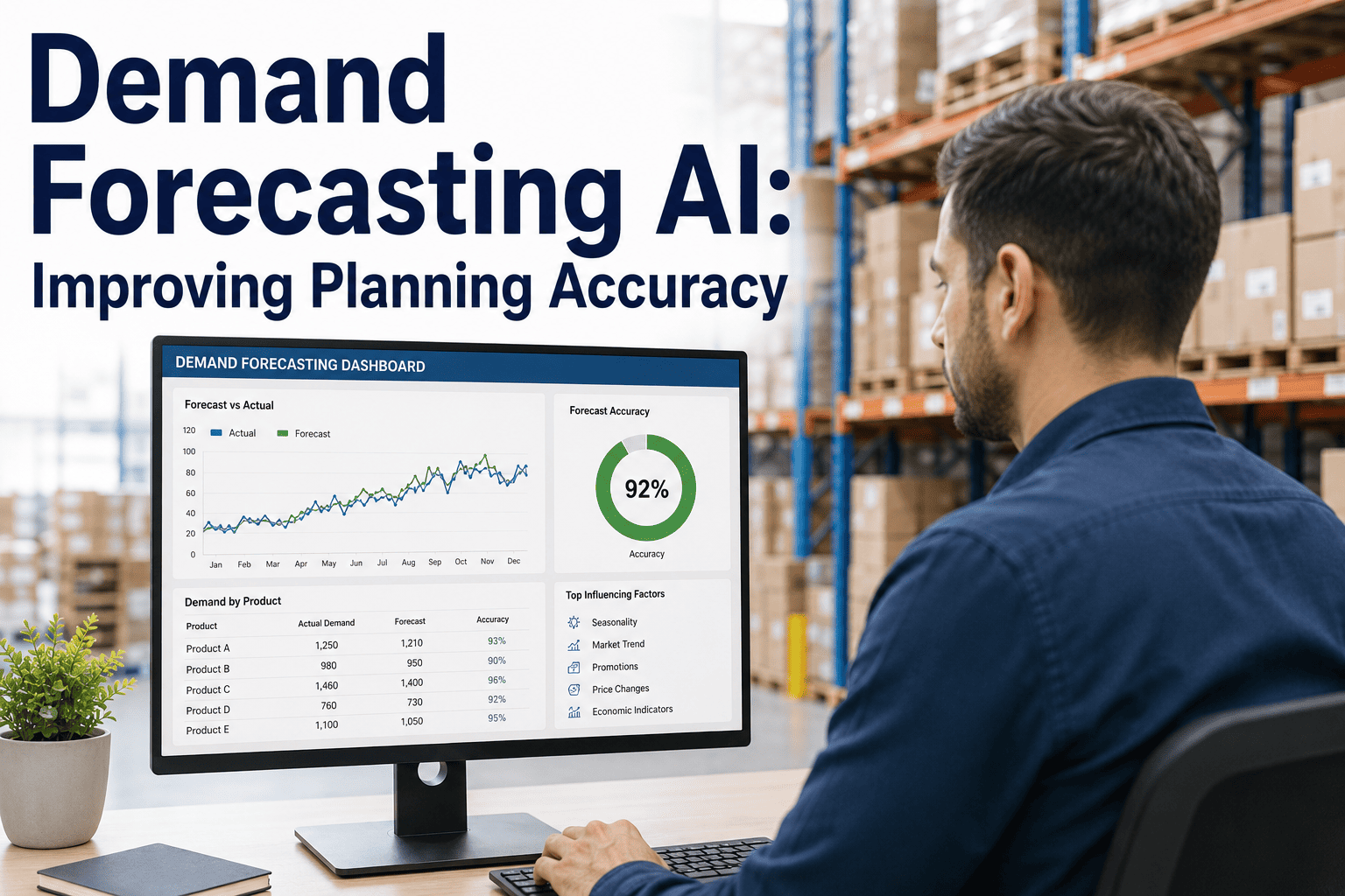
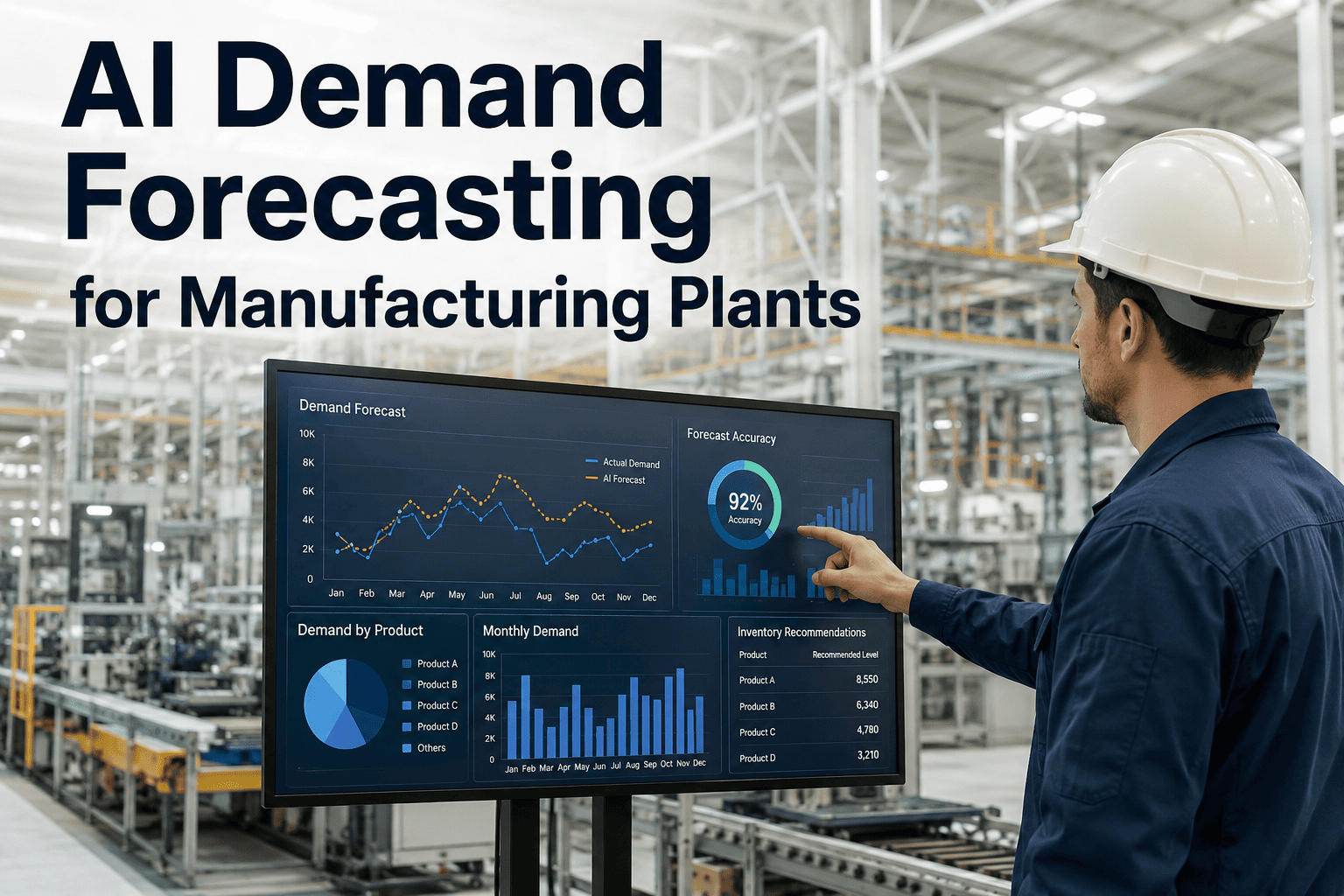
Manufacturing planners have relied on historical averages and spreadsheet-driven forecasts for decades, but the gap between what those methods predict and what actually hits the loading dock has only widened. Order patterns shifted during recent supply chain disruptions, customer lead times compressed, and SKU proliferation made simple time-series models unreliable at best. AI demand forecasting addresses this gap by giving planners a data foundation that matches the complexity of the actual demand signal, and plants report double-digit accuracy gains within two quarters. The downstream impact on inventory turns and schedule adherence is measurable from the first planning cycle — book a demo to see it applied to your demand history.
PRODUCTION PLANNING · DEMAND FORECASTING · AI ACCURACY
Demand Forecasting AI Is Rewriting How Manufacturing Planners Predict the Next Quarter
AI demand forecasting ingests your order history, customer behavior patterns, and external signals to produce forecasts that outperform traditional methods — directly feeding production schedules, procurement cycles, and inventory targets with measurable accuracy gains.
37%
Average Forecast Accuracy Improvement with AI
18 Days
Reduction in Planning Cycle Time
2.3x
Inventory Turn Improvement in Six Months
94%
Schedule Adherence Achieved by AI Plants
WHY SPREADSHEETS STOP WORKING
Traditional Forecasting Methods Were Built for a Market That No Longer Exists
The forecasting toolkit most manufacturing planners inherited — moving averages, exponential smoothing, seasonal decomposition — was designed for markets where demand followed recognizable patterns, lead times were stable, and the SKU count was manageable. None of those conditions hold for the majority of mid-market manufacturers today. The result is a planning process that looks rigorous on paper but consistently misses the actual demand signal by enough margin to drive expediting costs, excess inventory, and missed delivery dates across every quarter.
01
Moving Averages Collapse Under Volatility
A three-month moving average treats every data point in the window equally. When a major customer shifts ordering cadence — pulling forward Q3 orders into Q2 or splitting a large order across three months — the moving average smooths out the signal the planner most needs to see. By the time the adjusted average reflects the new pattern, the planning window has already closed and procurement is chasing material that should have been ordered weeks earlier. Plants running on moving averages during the 2021-2023 supply disruptions routinely carried 30 to 45 days of excess safety stock on the wrong SKUs while stockouting on the ones that actually moved.
02
Exponential Smoothing Cannot Handle Multiple Signals
Exponential smoothing improves on moving averages by weighting recent data more heavily, but it still models a single variable against time. In manufacturing, demand is driven by dozens of concurrent variables — customer pipeline changes, promotional calendars, competitor pricing shifts, macroeconomic indicators, and weather patterns for climate-sensitive products. A single-variable time-series model has no mechanism to ingest these signals, so the planner ends up applying manual overrides based on intuition. Those overrides are where institutional knowledge lives, but they are also where bias, inconsistency, and undocumented assumptions enter the forecast.
03
Spreadsheet Models Do Not Scale Past a Few Hundred SKUs
A planner managing 200 SKUs can maintain a separate forecast model for each product family and still review the outputs in a weekly meeting. At 2,000 SKUs — which is common for a mid-market fabricated metals or specialty chemicals plant — that approach breaks down. Models go unreviewed for months, assumptions compound, and the forecast becomes a self-referencing document that diverges further from reality with each planning cycle. The planner is not failing; the tool is being asked to do work it was never designed for. AI demand forecasting was built precisely for this scale problem.
THREE FORECASTING ARCHITECTURES
How AI Demand Forecasting Actually Works — Three Models Ranked by Complexity and Use Case
Not every AI demand forecasting approach is the same. The term covers a spectrum from statistical machine learning that extends traditional methods with feature engineering, through deep learning sequence models that learn temporal patterns directly from raw data, to hybrid ensembles that combine multiple model families with a planner-override layer. Choosing the wrong architecture for your demand profile is the most common reason AI forecasting projects underdeliver.
STATISTICAL MACHINE LEARNING
How It Works
Engineered features — lagged demand, rolling averages, price indices, promotional flags — are fed into gradient-boosted tree models or random forests that learn non-linear relationships between inputs and demand. The model does not see raw time-series data; it sees the features a data scientist or planner has constructed from that data.
Best For
Plants with 500 to 5,000 SKUs, moderate seasonality, and planners who can define the demand drivers. Feature engineering lets domain knowledge directly shape the model.
Limitation
Accuracy depends heavily on feature quality. If the planner misses a demand driver — a new customer contract, a competitor exit — the model has no way to discover it independently.
15-25%
Typical Accuracy Gain Over Baseline
DEEP LEARNING SEQUENCE MODELS
How It Works
LSTM or Transformer-based models ingest raw historical demand sequences and learn temporal patterns — seasonality, trend shifts, cyclic behavior — without manual feature engineering. Multi-variate versions can ingest external signals like commodity prices or weather data alongside demand history.
Best For
High-SKU environments with complex, multi-layered seasonality and rich external data sources. Deep learning excels when the demand pattern is too complex for a human to decompose into features.
Limitation
Requires large historical datasets — typically 36-plus months — and significant compute for training. Less interpretable than tree-based models, making it harder for planners to understand why a specific forecast was generated.
25-40%
Typical Accuracy Gain Over Baseline
HYBRID ENSEMBLE WITH PLANNER LAYER
How It Works
Multiple model families — statistical base, ML correction, deep learning overlay — generate independent forecasts. An ensemble layer weights each model's contribution by SKU, region, and time horizon. A final planner-override layer lets the demand planner adjust the ensemble output with documented reasoning that feeds back into model retraining.
Best For
Plants that need the highest achievable accuracy and want to preserve planner judgment as a governed, auditable input rather than an untracked override. This is the architecture used in most production-grade manufacturing forecasting deployments.
Limitation
Most complex to deploy and maintain. Requires ongoing model monitoring, ensemble weight tuning, and a change-management process for the planner override layer.
30-45%
Typical Accuracy Gain Over Baseline
HEAD-TO-HEAD COMPARISON
Demand Forecasting Methods Compared — From Spreadsheets to Hybrid AI
The table below compares six forecasting approaches across the dimensions that matter to a manufacturing planning team: data requirements, training and deployment timeline, typical accuracy range, and the situations where each method is the right choice. This is the comparison framework we walk through in the first session of every forecasting engagement.
| Approach |
Data Required |
Setup Time |
Accuracy Range |
Best Situation |
Key Limitation |
| Moving Average |
3-12 months history |
None |
60-70% MAPE |
Stable demand, low SKU count |
Collapses under volatility |
| Exponential Smoothing |
12-24 months history |
None |
65-75% MAPE |
Trend plus single-seasonality patterns |
Single variable only |
| ARIMA / SARIMA |
24-36 months history |
1-2 weeks |
70-78% MAPE |
Well-understood seasonal patterns |
Cannot ingest external signals |
| Statistical ML |
18-36 months plus features |
4-8 weeks |
78-88% MAPE |
Known demand drivers, mid-SKU range |
Feature quality dependent |
| Deep Learning |
36+ months raw sequences |
8-14 weeks |
82-92% MAPE |
Complex seasonality, rich data |
Large data and compute need |
| Hybrid Ensemble |
24+ months, multiple sources |
10-16 weeks |
85-95% MAPE |
Highest accuracy requirement |
Most complex to maintain |
Your Forecasting Method Should Match Your Demand Complexity — Most Plants Are Still Using a Method Built for Simpler Times
If your SKU count has grown, your customer mix has shifted, and your planning team is spending more time overriding forecasts than trusting them, the method is the problem. A structured assessment of your demand profile takes one session and shows exactly which AI architecture fits your operation.
FORECAST-TO-FLOOR CONNECTION
How an AI Demand Forecast Travels From Model Output to the Shop Floor Schedule
A more accurate forecast is worthless if it does not reach the systems that drive procurement, scheduling, and capacity allocation. The value of AI demand forecasting is realized only when the forecast number becomes a planning input that flows through the organization without manual re-entry, interpretation gaps, or version conflicts. The chain below shows the five stages an AI forecast passes through on its way to the shop floor, and where most plants lose accuracy in the handoffs.
01
Demand Signal Ingestion
Order history, open pipeline, customer portal data, distributor POS feeds, and external signals — commodity prices, housing starts, freight indices — are collected into a unified demand data lake. The ingestion layer normalizes time granularity, fills gaps, and tags data quality issues before any model sees the input. This stage is where most data quality problems surface: missing weeks, currency mismatches, and duplicate order entries that would corrupt the model if not caught here.
02
Forecast Generation
The ensemble model runs at a configured cadence — weekly for most manufacturing plants — generating SKU-level forecasts by week or by month across the planning horizon. Each model in the ensemble produces an independent forecast, and the weighting layer combines them. The output includes point forecasts, confidence intervals, and a model disagreement flag that highlights SKUs where the underlying models diverge — an early warning that the demand pattern is changing and the planner should investigate.
03
Planning Consensus
The demand planner reviews the AI forecast against qualitative inputs the model cannot see — a new customer contract, a competitor plant closure, a known one-time order. Adjustments are made through a governed override interface that records the planner's reasoning, the magnitude of the change, and the original model output. This is the critical handoff: the planner adds value the model cannot, and the model provides a baseline the planner would never achieve manually.
04
Schedule and Procurement Push
The consensus forecast feeds directly into the Master Production Schedule and MRP run. No re-entry, no spreadsheet bridge. Procurement lead times are calculated against the forecast, safety stock targets are adjusted based on forecast confidence intervals, and capacity planning uses the demand profile to identify bottleneck weeks. This is where accuracy translates to working capital: a 5-point MAPE improvement at this stage typically reduces safety stock by 15 to 20 percent on affected SKUs.
05
Execution Feedback Loop
Actual demand — orders received, shipments made, stockouts encountered — flows back into the model training pipeline. Forecast error is decomposed by SKU family, region, and time horizon to identify systematic biases. The ensemble weights are recalibrated monthly. The planner override log is analyzed to find patterns: if the planner consistently adjusts a specific product family upward, the model is underfitting that segment and the feature set needs review. This closed loop is what separates a deployed AI forecast from a one-time analysis.
ACCURACY METRICS
Four Forecast Accuracy Metrics That Tell You Whether Your AI Is Actually Working
Most manufacturing plants measure forecast accuracy with a single number — usually MAPE — and call it done. That single number hides more than it reveals. A plant can report a 15% MAPE while systematically over-forecasting high-volume SKUs and under-forecasting long-tail items, producing an aggregate number that looks acceptable while the planning team works around the model on both ends. The four metrics below give a complete picture of forecast performance and are the ones we track in every AI forecasting deployment.
MAPE
Mean Absolute Percentage Error
Measures the average percentage deviation between forecast and actual demand across all SKUs and periods. It is the most widely cited forecast accuracy metric in manufacturing and the one most planning teams are already tracking. MAPE is useful for headline comparison — before versus after AI deployment — but it has a known weakness: it over-penalizes errors on low-volume SKUs where a small absolute error produces a large percentage error. Use MAPE for executive reporting and trend tracking, but never as the sole accuracy measure.
Target: Below 20% for most manufacturing
WAPE
Weighted Absolute Percentage Error
Weights each SKU's error by its actual demand volume, so a 50-unit error on a 10,000-unit SKU counts proportionally more than a 50-unit error on a 200-unit SKU. WAPE is the metric that best reflects the operational impact of forecast error because it aligns error magnitude with revenue and inventory impact. A plant with a good MAPE but a bad WAPE is likely over-forecasting small SKUs and under-forecasting large ones — a pattern that drives excess inventory on the wrong products and stockouts on the ones that matter.
Target: Below 15% for volume-weighted accuracy
BIAS
Mean Error — Systematic Over or Under Forecasting
Unlike MAPE and WAPE, which measure the size of errors regardless of direction, bias tells you whether your forecast is systematically high or low. A positive bias means consistent over-forecasting — the plant is building inventory it does not need. A negative bias means consistent under-forecasting — the plant is missing orders and running overtime. Bias is the first metric to check after deployment because it reveals model calibration problems that MAPE masks. An AI forecast with low MAPE but high positive bias is generating numbers that look accurate on average but are systematically driving the wrong inventory decisions.
Target: Within plus or minus 3% of actual
FVA
Forecast Value Added — Does Each Step Improve the Number
FVA measures whether each step in the forecasting process — statistical baseline, ML adjustment, planner override, management review — makes the forecast more or less accurate. If the planner's overrides consistently increase error relative to the model baseline, the override process is destroying value. If management review shifts the forecast further from actual, the review step is adding noise. FVA is the metric that drives organizational change because it makes the cost of each process step visible and quantifiable. Plants that track FVA typically find that 20 to 30 percent of planner overrides degrade accuracy.
Target: Every process step adds positive value
IMPLEMENTATION PITFALLS
Seven Mistakes That Cause AI Demand Forecasting Projects to Underdeliver
AI demand forecasting has a high success rate when deployed correctly, but a significant share of projects fail to deliver the accuracy gains the business case promised. In almost every case, the failure is not in the model — it is in the deployment approach. The seven mistakes below are the ones we see most often in manufacturing forecasting engagements, and each one is avoidable with the right project structure.
01
Starting With the Full SKU Catalog Instead of a Pilot Segment
Teams that try to forecast all 3,000 SKUs in the first deployment spread data science resources too thin, delay time to value, and make it impossible to isolate problems. The correct approach is to select a pilot segment — a product family with 100 to 300 SKUs, known demand drivers, and a planning team willing to engage — prove accuracy gains there, and then extend. A successful pilot creates internal advocates and a template for the broader rollout.
02
Skipping the Demand Driver Interview With the Planning Team
Data scientists who build forecasting models without talking to the people who currently own the forecast will miss critical demand drivers that do not appear in any data system. The planner knows that Customer A always doubles orders before their fiscal year-end, that Product B demand is tied to a specific regulatory filing deadline, that Region C is losing share to a new competitor. These are not in the ERP. If they are not captured as features or override rules, the model will never learn them.
03
Not Building a Planner-in-the-Loop Override Layer From Day One
AI forecasts that are dropped into the planning process without an override mechanism create two problems: planners either ignore the forecast and work around it, or they make undocumented adjustments in spreadsheets that break the feedback loop. The override layer must be designed into the system from the start — a simple interface where the planner can adjust the forecast, record the reason, and have that adjustment flow back into model evaluation. This is not a nice-to-have; it is the mechanism that makes the AI forecast a planning tool rather than a report.
04
Treating the Forecast as a Set-and-Forget System
Demand patterns drift. Customer mixes shift. New products launch. Competitors enter and exit. An AI forecast that is not retrained and recalibrated monthly will degrade at a rate that surprises most teams — accuracy can drop 5 to 10 points in a single quarter if the model is not seeing fresh data. The deployment must include a retraining cadence, an ensemble weight recalibration schedule, and a monitoring dashboard that flags accuracy degradation before it becomes a planning problem.
05
Measuring Only MAPE and Ignoring Bias and FVA
A single accuracy metric creates a false sense of security. Plants that track only MAPE often discover — too late — that the model is systematically over-forecasting one segment and under-forecasting another, producing an aggregate number that hides operational problems. Bias and FVA must be part of the monitoring suite from the first week of deployment. If you are not tracking whether each step in your process adds or destroys forecast value, you cannot improve the process.
06
Skipping the Data Quality Audit Before Model Training
Garbage in, garbage out is not a cliché in demand forecasting — it is the primary failure mode. Duplicate order entries, missing weeks in the history, currency mismatches between domestic and export orders, and promotional orders tagged as regular demand will all corrupt the model. The data quality audit — a structured review of completeness, consistency, and correctness across the demand history — should consume 30 to 40 percent of the project timeline in the first deployment. Teams that rush this step spend the rest of the project debugging model outputs that are actually data problems.
07
Not Connecting the Forecast Output to MPS and MRP Systems
An AI forecast that lives in a separate dashboard and requires manual re-entry into the ERP planning module will never achieve its intended impact. The integration path — forecast output to Master Production Schedule input, safety stock recalculation triggers, and procurement lead-time adjustment — must be designed in the architecture phase, not deferred to a later phase. Every manual handoff is a point where accuracy is lost, timing is delayed, and the planning team loses trust in the AI output.
FREQUENTLY ASKED QUESTIONS
What Manufacturing Planning Teams Ask Before Adopting AI Demand Forecasting
How is AI demand forecasting different from the forecasting module already built into our ERP system?
ERP forecasting modules typically implement statistical methods — moving averages, exponential smoothing, or at most a basic regression — that were state-of-the-art twenty years ago. They run on a single demand variable, cannot ingest external signals, and do not learn from forecast errors over time. AI demand forecasting uses machine learning and deep learning models that process multiple demand drivers simultaneously, detect complex non-linear patterns, and improve through a continuous feedback loop. The difference is not incremental — plants that switch from ERP-native forecasting to AI models typically see 15 to 40 percent accuracy improvement depending on demand complexity.
Book a demo to see a side-by-side comparison using your actual demand data.
How much historical data do we need before AI demand forecasting produces reliable results?
Statistical ML models can produce useful results with 18 to 24 months of clean demand history, while deep learning sequence models typically require 36 or more months to learn seasonal and cyclical patterns effectively. The more important variable than raw volume is data quality — 24 months of clean, deduplicated, correctly tagged order history will outperform 48 months of messy data every time. In the first engagement, we spend significant time on the data quality audit precisely because the model's ceiling is set by the data, not by the algorithm.
Talk to our support team about a data readiness assessment for your demand history.
Does AI demand forecasting replace our demand planners or change their role?
No. The AI replaces the mechanical part of the forecasting process — calculating baselines, detecting patterns, flagging anomalies — and frees the planner to focus on the parts that require human judgment: interpreting market shifts, incorporating customer relationship intelligence, and making strategic override decisions. In every successful deployment, the planner's role shifts from building forecasts in spreadsheets to reviewing and adjusting AI-generated forecasts through a governed interface. The planner's domain knowledge becomes more valuable, not less, because the AI provides a better baseline to adjust from and the override layer documents every decision for audit and training.
Book a demo to see the planner workflow in a live forecasting environment.
How do we handle new product introductions that have no demand history for the model to learn from?
New products are forecasted using attribute-based models that map the new product to the demand profile of similar existing products based on shared attributes — product family, customer segment, price point, geography, and channel. When a new SKU launches, the system identifies the nearest historical analogs, generates a baseline forecast from their demand curves, and flags the SKU as a new-product forecast with lower confidence intervals. As actual demand comes in, the model transitions from attribute-based forecasting to history-based forecasting over a defined ramp-up period. This approach typically achieves 70 to 80 percent of the accuracy of a mature SKU forecast within the first two months of a new product launch.
Contact support to discuss new-product forecasting approaches for your product architecture.
What happens when the AI forecast is significantly wrong — how do we prevent planning disruption?
The AI forecast includes confidence intervals that tell the planner how certain the model is about each SKU-level prediction. When confidence drops below a configured threshold — because of demand pattern changes, missing data, or model disagreement within the ensemble — the system flags the SKU for mandatory planner review before the forecast enters the planning pipeline. The planner-in-the-loop override layer is specifically designed for this scenario: the AI surfaces its uncertainty, the planner applies judgment, and the override is logged with reasoning. The forecast never enters MPS or MRP without passing through this checkpoint. Additionally, the feedback loop captures the error, decomposes it, and uses it to improve the model for the next cycle.
Book a demo to see how the confidence interval and override workflow operates in practice.
SEE IT ON YOUR DEMAND DATA
Your Planning Team Deserves a Forecast That Matches the Complexity of Your Actual Demand
An AI demand forecasting assessment mapped to your SKU catalog, customer mix, and planning cycle takes one session — and shows exactly where your current method is losing accuracy and what an AI model would recover. The forecast improvement is quantified before any commitment is made.