A reservoir engineer covering 300 wells across a basin used to spend the first week of every quarter re-fitting Arps decline curves one well at a time — pulling monthly rates, eyeballing the hyperbolic exponent, adjusting b-factors that did not quite match what the well was actually doing, then rolling the individual estimates up into a type curve nobody fully trusted. Machine learning production forecasting replaces that quarterly ritual with a model that retrains itself continuously against every well in the field, catching production shifts within days instead of waiting for the next manual review. Reserve estimates that once took a week of curve-fitting now update automatically as new data arrives, and the accuracy gap against traditional decline curves has become too large for asset teams to ignore. Book a demo to see production forecasting configured against your own type curves.
PRODUCTION FORECASTING · MACHINE LEARNING · EUR ACCURACY
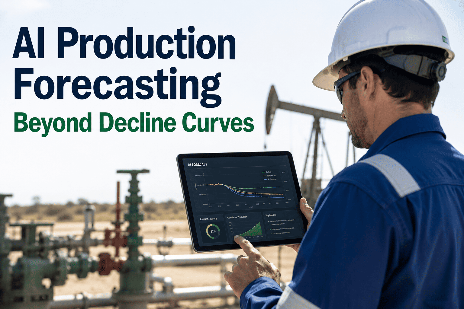
AI Production Forecasting That Goes Beyond the Decline Curve — Sharper EUR, Faster Updates, Fewer Surprises
Machine learning production forecasting folds reservoir properties, completion design, and operating history into the same model that used to rely on a single production trend line — replacing static, manually-refit Arps curves with forecasts that update automatically and hold up better against actual field performance.
20–30%
More Accurate EUR Estimates Than Arps Decline Curves Alone
20+
Geological, Completion, and Operating Inputs Used Per Well Forecast
Daily
Forecast Refresh vs Quarterly Manual Curve-Fitting Cycles
THE DECLINE CURVE LIMITATION
Why Arps Decline Curves Run Out of Room in Complex Unconventional Fields
Arps decline curve analysis has been the industry standard since the 1940s because it is simple, transparent, and fast — fit three parameters to a production history and extrapolate forward. That simplicity is also its ceiling. Arps treats every well as an isolated time series, ignoring reservoir quality, completion intensity, and parent-child spacing effects that increasingly dominate well performance in shale and tight formations. Two wells with identical decline curves in year one can diverge sharply by year three once interference from an offset well or a change in choke management shows up — and a curve fit purely to historical rate has no way to see that coming.
The practical cost shows up at the portfolio level. A reservoir engineering team refitting curves manually every quarter is working from data that is already stale by the time the type curve is published, and dynamic updates require the same manual rework every cycle. Independent studies comparing machine learning approaches against Arps baselines have found accuracy improvements in the 20 to 30 percent range once the model is given access to geospatial, petrophysical, drilling, and completions data rather than production history alone — because the extra predictors capture exactly the well-to-well variation that a single decline curve cannot.
HOW IT WORKS
The Four-Stage Pipeline Behind Machine Learning Production Forecasting
Machine learning production forecasting is not a single algorithm replacing Arps — it is a pipeline that ingests a much wider set of inputs, engineers features an engineer would not manually track across hundreds of wells, and blends multiple model types to produce a forecast with a defensible uncertainty range.
01
Data Ingestion — Production, Completion, and Reservoir Records
Monthly oil, gas, and water rates, bottom-hole pressures, and cumulative volumes are pulled alongside completion design, lateral length, proppant intensity, and offset well spacing for every well in the analog set.
02
Feature Engineering — Turning Raw History Into Model Inputs
Decline parameters from a conventional Arps fit — initial rate, nominal decline, hyperbolic exponent — are calculated and retained as inputs rather than discarded, giving the model a physics-grounded starting point to refine.
03
Model Ensemble — Gradient Boosting, Neural Networks, and Sequence Models
Gradient-boosted trees, artificial neural networks, and sequence models such as LSTM or GRU are trained and cross-validated against held-out wells, each contributing a forecast that is blended into a single ensemble output.
04
Type Curve & EUR Output — Continuously Refreshed
The ensemble produces a well-level and type-curve forecast with an uncertainty band, refreshed as new production months land — no manual re-fit required to keep the reserve estimate current.
TRADITIONAL VS MACHINE LEARNING
Arps Decline Curve Analysis Compared Against Machine Learning Forecasting
Both approaches produce a production forecast and an EUR number, but they get there through fundamentally different mechanics — and that difference shows up directly in accuracy, refresh speed, and how well the forecast holds up as a field matures.
| Dimension | Arps Decline Curve | Machine Learning Forecast |
| Inputs used |
Single well production history |
20+ geological, completion, and operating variables |
| Update cycle |
Manual re-fit, typically quarterly |
Automatic refresh as new data lands |
| Parent-child interference |
Not captured |
Learned from analog well behavior |
| Typical EUR accuracy gain |
Baseline |
20–30% improvement over Arps baseline |
| Uncertainty range |
Deterministic single curve |
Probabilistic band with confidence intervals |
| Analyst effort per cycle |
Hours per well across the portfolio |
Minutes to review flagged wells |
DASHBOARD VIEWS
Who Uses the Forecast — and What Each Role Actually Needs to See
A production forecasting platform is not one screen. A reservoir engineer wants the well-level fit and residuals. An asset team lead wants the type curve rolled up by pad. A reserves analyst wants the number that feeds the PRMS category. The same underlying model serves all three from one data set.
Reservoir Engineer
Well-level forecast vs actual with residual tracking
Feature importance for each well's forecast drivers
Flagged wells where actual diverges from prediction
Asset Team Lead
Type curve by pad, landing zone, and completion vintage
Portfolio EUR roll-up with confidence bands
Parent-child interference flags for infill planning
Reserves & A&D Analyst
PRMS-aligned P90/P50/P10 reserve categories
Forecast audit trail for reserve report support
Comparative screening across acquisition targets
Executive / Portfolio Owner
Field-level production outlook, 12 and 24 month
Forecast accuracy tracked against realized production
Capital allocation signals from type curve shifts
A Forecast That Updates Itself Is Worth More Than One That Just Looks Accurate on the Day It Was Built
Continuous retraining, uncertainty bands that hold up under audit, and a forecast that reflects this month's data instead of last quarter's curve fit.
WHAT FEEDS THE MODEL
The Data a Machine Learning Forecast Uses That a Decline Curve Never Sees
The accuracy gain over Arps does not come from a smarter curve-fitting algorithm — it comes from giving the model access to information a single-well decline curve structurally cannot use. Every one of the categories below has been shown in published studies to carry predictive signal for future production that pure rate history misses.
01
Geological & Petrophysical Properties
Porosity, permeability, total organic carbon, and reservoir pressure by landing zone, pulled from logs and offset well analogs rather than assumed constant across the field.
02
Completion Design Parameters
Lateral length, stage count, proppant and fluid intensity per foot, and cluster spacing — the variables that explain why two offset wells with similar geology can produce very differently.
03
Parent-Child Spacing & Sequencing
Distance to offset wells and the order in which they were drilled and completed, which drives interference effects that a single-well decline curve has no mechanism to represent.
04
Operational & Field Conditions
Choke management history, artificial lift changes, shut-in events, and facility constraints — day-to-day operating decisions that shift a well off its baseline decline trajectory.
RESERVE CONFIDENCE
How Probabilistic Forecasting Supports PRMS Reserve Categories
Reserve reporting under the Petroleum Resources Management System requires low, best, and high estimates — P90, P50, and P10 — reflecting a defensible range of uncertainty rather than a single deterministic number. A machine learning forecast trained with cross-validation naturally produces a probability distribution around its prediction, which maps directly onto these reserve categories instead of requiring a separate manual sensitivity exercise layered on top of a single Arps curve.
That matters most at the point of an audit or a reserve report review, where the forecast needs to show its work: which wells drove the estimate, how the model performed against realized production in prior periods, and how the uncertainty band was derived. A continuously validated model carries that audit trail automatically, updated with every retraining cycle rather than reconstructed by hand each reporting period.
MODEL SELECTION
Which Machine Learning Model Fits Which Forecasting Scenario
There is no single model architecture that wins across every field type, which is why most production-grade forecasting deployments blend several model families rather than betting the reserve estimate on one algorithm. Each family below has a distinct strength, and the ensemble output typically weights them according to how well each one performed on the specific well population being forecast.
A
Gradient-Boosted Trees (XGBoost, LightGBM)
Best where geological and completion inputs dominate the forecast — fast to retrain across large well populations and transparent enough to rank which input features are driving each well's prediction.
B
Artificial Neural Networks & Support Vector Regression
Effective at capturing nonlinear relationships across a high-dimensional input set, particularly once dozens of geological and operating predictors are in play, though they typically need a larger training set to avoid overfitting.
C
LSTM & GRU Sequence Models
Purpose-built for the temporal pattern in the decline itself, and reported in published comparisons to outperform conventional decline models in tight gas and unconventional settings when trained with enough well history.
D
Prophet & Seasonal-Trend Decomposition
Well suited to wells with shut-ins or irregular production patterns, including enhanced oil recovery applications, where standard decline curves struggle to fit the interruptions cleanly.
FREQUENTLY ASKED QUESTIONS
Questions Reservoir and Reserves Teams Ask About Machine Learning Forecasting
Does machine learning forecasting replace Arps decline curve analysis entirely?
No — the decline parameters from an Arps fit are typically retained as one of the model's input features rather than discarded, because they carry genuine physical signal about a well's early-time behavior. What changes is that the model no longer relies on that single curve alone; it blends the Arps fit with geological, completion, and offset-well data to correct for the interference and reservoir-quality effects a decline curve cannot see on its own.
Book a demo to see how the two approaches work together on your well set.
How much data history is needed before a machine learning forecast becomes reliable?
Models are typically trained across the full analog set for a play — often hundreds of wells with at least twelve to twenty-four months of production history — rather than a single well in isolation. A new well with only a few months of data can still be forecast reasonably well because the model borrows strength from similar wells elsewhere in the training set, an approach that pure single-well curve fitting cannot replicate.
Contact forecasting support to review data requirements for your field.
Can the forecast account for a well that goes through an artificial lift conversion or workover?
Yes, provided the operational event is captured in the input data. Because the model ingests operating history alongside production rates, a lift conversion, choke change, or workover shows up as a feature the model can learn from — and the forecast adjusts on the next retraining cycle rather than waiting for a manual re-fit to catch the shift.
Book a session to walk through how operational events are incorporated.
How is forecast accuracy validated before it is used for reserve reporting?
Models are validated using cross-validation against held-out wells and tracked using standard error metrics such as mean absolute error and root mean square error, compared against both the training set and subsequent realized production. That validation history becomes part of the audit trail a reserves team can present alongside the reported P90/P50/P10 estimates.
Talk to support about validation reporting for audit purposes.
Does this approach work for conventional wells, or only unconventional shale plays?
The parent-child interference and completion-intensity features are most valuable in unconventional plays where well spacing and completion design vary widely, but the underlying pipeline — ensembling a decline-curve baseline with reservoir and operational data — applies to conventional production forecasting as well, particularly for fields with strong offset-well analog data available.
Book a demo to discuss your specific field type.
SHARPER EUR · FASTER UPDATES · AUDIT-READY
Replace the Quarterly Curve-Fitting Cycle With a Forecast That Keeps Itself Current
See a machine learning production forecast built against your own type curves, completion data, and offset well set — with the uncertainty bands your reserves team needs.





.png)