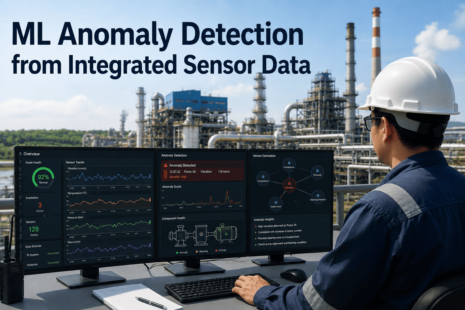
Power plant monitoring systems generate thousands of alarms per day across distributed control systems, vibration monitoring platforms, emissions analyzers, and electrical protection relays — yet the vast majority of these alarms are either nuisance alerts that operators have learned to ignore or redundant notifications that arrive after an event has already progressed beyond the point where early intervention was possible. Machine learning anomaly detection changes this dynamic by ingesting data from all of these sensor systems simultaneously, learning the normal correlated behavior patterns that exist between process variables, vibration signatures, and electrical parameters, and flagging only the deviations that represent genuine emerging faults rather than routine process variations. You can book a demo to see how cross-system ML anomaly detection works against unified power plant sensor data.
Why Power Plant Alarm Systems Produce Noise Instead of Insight
The ISA-18.2 alarm management standard identifies alarm flooding — defined as more than ten alarms per ten-minute period per operator — as a primary indicator of an ineffective alarm system. In practice, many power plants significantly exceed this threshold during routine operating transitions such as load changes, startup sequences, and fuel switches, with some units generating hundreds of alarms per hour during periods that are not genuinely abnormal but simply involve process variables moving through threshold zones that were configured as fixed setpoints without accounting for the normal dynamic relationships between variables. The result is an alarm environment where operators cannot reliably distinguish between a genuinely abnormal developing fault and a routine process variation that happens to have crossed a threshold boundary.
This problem is fundamentally a consequence of how traditional alarm systems evaluate each sensor measurement independently. A bearing temperature alarm triggers when the temperature exceeds a fixed setpoint. A vibration alarm triggers when amplitude exceeds a fixed threshold. An electrical current alarm triggers when draw exceeds a fixed limit. Each of these individual thresholds may be perfectly reasonable when evaluated in isolation, but none of them account for the operating context — whether the unit is at full load or low load, whether ambient conditions are affecting cooling effectiveness, whether a recent operational change has shifted the normal baseline for that measurement. The alarm system treats every variable as if it operates in a vacuum, which is precisely the opposite of how an actual power plant works, where every process variable is connected to every other variable through thermodynamic, mechanical, and electrical relationships.
The economic impact of this alarm noise extends beyond operator fatigue. When alarms are predominantly nuisance events, operators develop a rational response pattern of acknowledging and dismissing them quickly, which means that when a genuine fault does produce an alarm, it arrives in a context where the operator has been trained by experience to expect that most alarms do not represent real problems. This is not an operator performance issue — it is a system design issue. The alarm system is asking operators to perform a pattern recognition task that the system itself is not performing: distinguishing between normal variation and abnormal deviation. Machine learning anomaly detection addresses this by moving the pattern recognition burden from the operator to the analytical system, where it belongs.
Why Monitoring Each Sensor System in Isolation Misses the Faults That Matter Most
Consider a developing bearing fault on a forced draft fan motor. In the early stages of degradation, the bearing may produce a subtle change in vibration signature — a slight increase in specific frequency components that falls well below the alarm threshold. Simultaneously, the increased friction may cause the motor current draw to shift by a small amount that is within the normal range for load variations. The bearing temperature may increase by a degree or two, which is within the deadband of the temperature alarm and also within the range of normal ambient variation. None of these individual changes is large enough to trigger an alarm in any single monitoring system. But the correlated pattern — vibration shifting in a specific direction, current adjusting in a complementary way, temperature trending upward in a manner consistent with increased friction — represents a clear anomaly when all three signals are evaluated together, even though no individual signal crosses any threshold.
This is the fundamental limitation of single-system monitoring: it can only detect faults that are severe enough to produce a threshold-crossing signal in one specific measurement type. Faults that manifest as distributed, correlated changes across multiple measurement types — which is how many real-world faults behave in their early stages — are invisible to a monitoring architecture that evaluates each system independently. The fault is happening, the data exists to detect it, but the analytical framework is not structured to see it because the relevant signals live in different systems that never communicate with each other during the analysis process.
The correlation matrix above illustrates why single-system monitoring has structural blind spots. A bearing degradation fault produces strong signals in vibration and current but minimal signals in pressure and flow. A valve stiction fault produces almost no signal in vibration, temperature, or current — but it produces strong signals in pressure and flow behavior. A monitoring system that only watches vibration will catch bearing faults early but will be essentially blind to valve stiction until the valve fails completely and the process variable it controls goes out of range. Only a monitoring approach that evaluates all of these signal types simultaneously can provide comprehensive fault coverage across the full range of failure modes that matter in a power plant environment.
How Machine Learning Detects Anomalies Differently Than Fixed Threshold Alarms
Traditional alarm systems compare individual measurements against fixed thresholds that are typically set during commissioning and adjusted only when nuisance alarm complaints become severe enough to trigger a review. Machine learning anomaly detection operates on a fundamentally different principle: instead of checking whether a single variable has crossed a line, it checks whether the overall pattern of behavior across many correlated variables has deviated from the learned normal operating envelope. This distinction — evaluating patterns rather than points — is what gives ML-based detection its ability to catch faults that fixed thresholds miss while simultaneously suppressing alarms that fixed thresholds generate unnecessarily.
The normal behavior model is the core of the system. During a training period — typically several weeks to several months of historical data covering the full range of normal operating conditions including load changes, startups, shutdowns, and seasonal variations — the ML algorithm learns the multivariate statistical structure of normal plant behavior. It learns that when load increases by 50 megawatts, main steam temperature typically increases by a certain amount, reheat spray flow adjusts in a predictable direction, condenser vacuum changes in a correlated way, and so on across hundreds or thousands of variable relationships. This learned structure becomes the reference against which new data is continuously compared.
When new data arrives, the model does not check whether any individual variable is outside its historical range. Instead, it checks whether the overall pattern of relationships between variables is consistent with the learned normal structure. A load change that produces the expected pattern of correlated responses across all variables produces a low anomaly score even though many individual variables have moved significantly. A subtle fault that causes one variable to shift in a direction that is inconsistent with the expected correlated response — even if that variable has not moved outside its historical range — produces a high anomaly score because the pattern is wrong, not because any single value is wrong.
This pattern-based approach is what enables the simultaneous reduction in false alarms and improvement in early detection. False alarms are reduced because normal process variations that cross fixed thresholds do not produce high anomaly scores when the correlated pattern is consistent with learned normal behavior. Early detection is improved because emerging faults that have not yet driven any single variable outside its normal range do produce high anomaly scores when the correlated pattern begins to deviate from the learned structure, often days or weeks before any fixed threshold would have been crossed.
What ML Catches That Single-System Monitoring Misses — Concrete Power Plant Examples
The theoretical advantages of cross-system ML anomaly detection become concrete when examined against specific fault scenarios that power plants actually experience. The following examples illustrate how faults that would be invisible or delayed under single-system monitoring are detected early when ML evaluates the correlated behavior of multiple sensor systems simultaneously.
In each of these scenarios, the underlying fault is the same. What changes is the analytical framework evaluating the data. Single-system monitoring evaluates each measurement against a fixed line and misses the fault because the fault has not yet pushed any single measurement across that line. Cross-system ML monitoring evaluates the pattern of relationships between measurements and catches the fault because the pattern has changed in a way that is inconsistent with normal behavior, even though every individual measurement remains within its normal range. The data is identical. The detection capability is fundamentally different.
Fixed Alarms vs. Adaptive ML Detection — Behavioral Differences Across Operating Conditions
Understanding why ML anomaly detection outperforms fixed threshold alarms requires examining how each approach behaves across the range of conditions a power plant actually experiences. Fixed thresholds are static — they do not change based on load, ambient conditions, fuel quality, or equipment condition. The alarm setpoint for a bearing temperature is the same at 100 percent load on a 95-degree day as it is at 40 percent load on a 40-degree night, even though the normal operating temperature for that bearing may differ by 15 degrees between those two conditions. ML detection is adaptive — the learned normal behavior model inherently accounts for these operating condition dependencies because the training data included all of these conditions, and the model learned what normal looks like at each point in the operating envelope.
The three scenarios above illustrate the core behavioral difference. Fixed thresholds produce false alarms when operating conditions push normal measurements close to the threshold boundary, miss genuine anomalies when operating conditions push abnormal measurements away from the threshold boundary, and generate alarm floods during normal transients because the thresholds were not designed for dynamic conditions. ML adaptive detection avoids all three failure modes because it evaluates whether the current behavior pattern is consistent with what it has learned is normal for the current operating context, rather than comparing individual values against lines that do not account for context.
This does not mean that fixed thresholds have no role in a modern monitoring architecture. Fixed thresholds serve an important safety function as hard limits that must never be exceeded regardless of the operating context — absolute maximum temperatures, pressures, and vibration levels that represent equipment protection limits. The most effective monitoring architecture uses ML anomaly detection as the primary early-warning system for identifying developing faults, with fixed thresholds retained as a separate, independent safety layer that activates only when an absolute limit is approached regardless of what the ML model says. This layered approach provides both the sensitivity of adaptive detection and the certainty of hard safety limits. Book a demo to see how ML detection and fixed threshold layers coexist in a unified monitoring architecture.
How ML Anomaly Detection Deploys Across Existing Power Plant Data Infrastructure
Deploying ML anomaly detection does not require replacing existing monitoring systems or control infrastructure. The ML platform sits alongside existing systems as an additional analytical layer that reads data from them without modifying their operation. This architectural approach means that existing DCS alarms, vibration system alerts, and protection relay functions continue to operate exactly as they do today — the ML system adds a new detection capability on top of the existing infrastructure rather than substituting for it. The deployment follows a structured sequence that progressively adds data sources and refines the model as the system gains experience with the specific operating characteristics of each plant.
A critical aspect of the deployment that is often underestimated is the data quality validation in Phase 1. Power plant historians frequently contain sensor failures, communication dropouts, frozen values, and calibration drift events that occurred during normal operations and were never corrected in the historical record. If these data quality issues are not identified and handled before model training, the ML algorithm will learn these artifacts as part of normal behavior, which degrades detection sensitivity and can produce model behavior that does not align with engineering expectations. Investing time in data quality assessment before training — typically two to four weeks for a major generating unit — pays significant dividends in model accuracy and engineering trust throughout the life of the deployment.