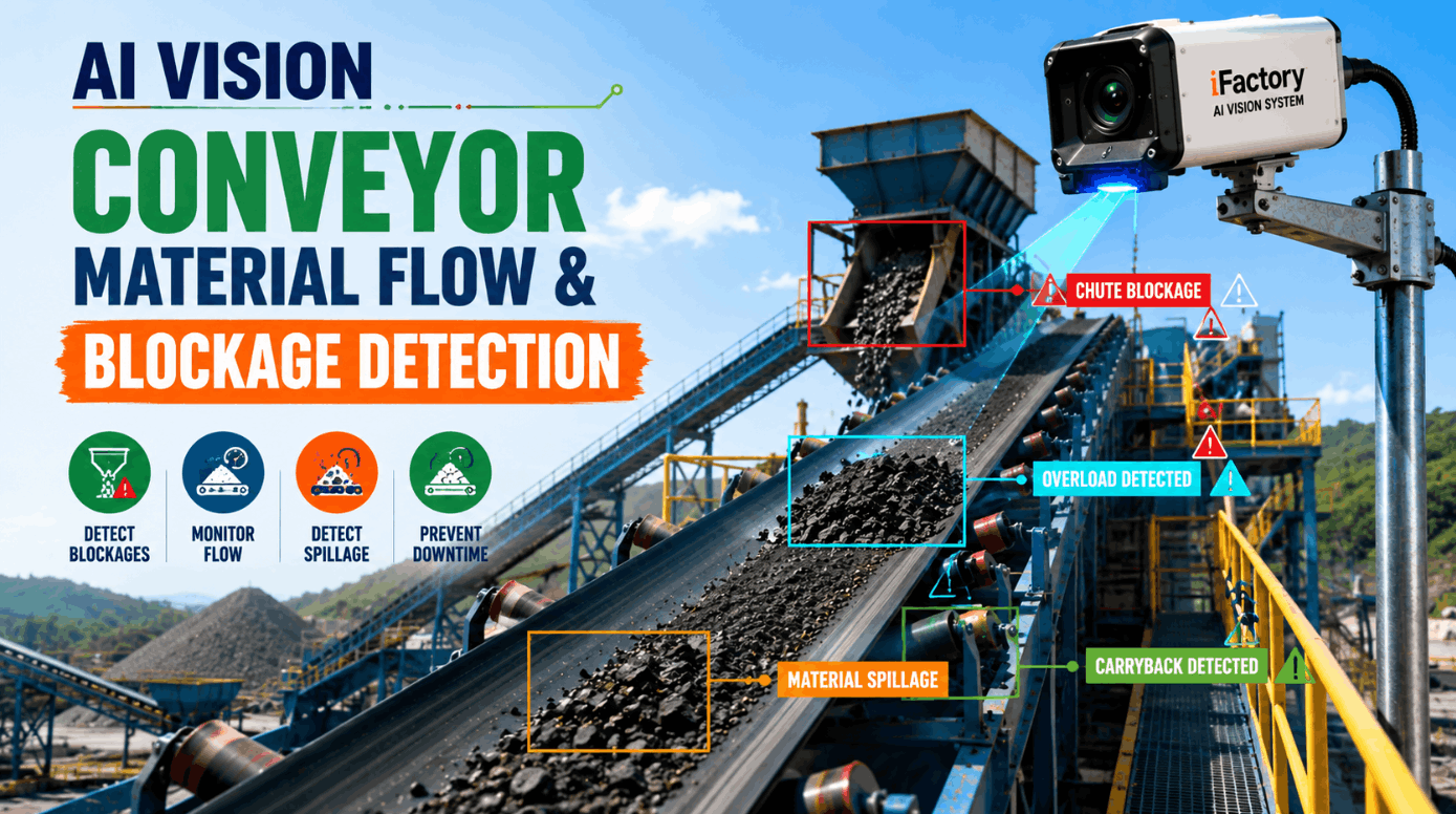
Every conveyor moving bulk material in 2026 is running blind in one dimension that matters more than any other: the volumetric shape of what is actually on the belt at any given moment. Traditional belt scales tell you tonnage. Level sensors tell you present or absent. Neither tells you whether the material is centred on the belt, whether the load profile is stable or surging, whether a chute is starting to plug, or whether the belt is running at 40% of capacity while the drive motor is burning full power. AI vision closes that gap by continuously profiling material load across the belt cross-section, measuring volumetric flow rate visually, and detecting surges, dips, misloads, and blockages before they cascade into downstream downtime. For plant operations leaders in mining, cement, steel, aggregate, and bulk handling, this is the single biggest instrumentation upgrade available in 2026 — plants ready to see it running on their own belts can book a demo and walk through a live load profile with the iFactory team.
MATERIAL FLOW · CONVEYOR LOAD PROFILE · VOLUMETRIC VISION · 2026
See What Your Belt Is Actually Carrying — Every Second
Vision cameras profile load across the belt cross-section, measure volumetric flow rate, and flag surges, dips, misloads, and developing blockages in real time. Optimise feeder rates. Protect motor loads. Stop losing capacity to guesswork.
97%+
Volumetric Accuracy
Achievable with vision plus 3D stereo or time-of-flight sensing against calibrated reference loads
40%
Belt Edge Wear Reduction
Reported when loading profile is optimised from vision-driven feeder adjustments
Continuous
Coverage Across kms of Belt
Vision replaces hours-apart manual inspection with 24/7 profile monitoring
Under 5s
Surge Detection Response
Vision-driven feeder throttle response to prevent chute overload downstream
Why Load Profile Beats Total Tonnage Every Time
A belt scale reports one number: how much mass crossed the sensor in the last second. That number can look perfectly healthy while the belt is actually running dangerously off-centre, surging every few seconds, or feeding a chute that is one bad minute away from plugging. The load profile — the actual shape of the material bed across the belt width and along the belt length — carries information the tonnage number physically cannot. It shows whether the load is centred, whether it is uniformly distributed or hollowed out in the middle, whether surge peaks are hitting three times the average, and whether the belt is running loaded to design capacity or wasting 30% of its throughput window.
This is where AI vision changes the conversation. A camera watching the belt cross-section, combined with either 3D stereo imaging, a laser line projector, or a time-of-flight sensor, reconstructs the material profile 20 or 30 times a second. The AI layer then does what a belt scale cannot: it classifies the profile as normal, surging, dipping, off-centre, or degrading toward a blockage — and feeds that classification back to the feeder control loop or the CMMS. The belt scale tells you what happened. The vision system tells you what is about to happen.
The Four Load Conditions Every Belt Cycles Through
Any belt in continuous operation moves through the four load conditions below on a regular basis. Belt scales cannot distinguish between them because the tonnage signal often looks similar. Vision can, because it sees the geometry. Understanding these four conditions is the foundation of every load-profile optimisation programme.
What makes these four conditions worth naming and monitoring separately is that each one demands a different operator response. An optimal load requires no intervention. A surging load calls for a feeder rate adjustment or upstream bin agitation to break bridging. An off-centre load requires a chute or skirt alignment check. A developing blockage requires an immediate feeder slowdown and often a maintenance work order raised for a physical inspection at the next shift change. Treating them as one generic anomaly loses the specificity operations teams need to respond correctly, which is exactly why traditional threshold-based alarming on belt scales produces so many nuisance alerts. Vision-based classification turns a single anomaly signal into four actionable states, and that is where operational value starts to compound.
CONDITION A
Optimal Load
Material centred on belt at design capacity, uniform profile along belt length, smooth surface without visible surging. Drive motor loaded to nameplate, belt edge wear minimal.
Action: Maintain feeder rate
CONDITION B
Surging Load
Repeated peak-and-trough pattern in load profile, often driven by upstream bin bridging or feeder inconsistency. Drive motor experiences repeated overload spikes even when average tonnage looks normal.
Action: Trigger feeder adjustment, alert operator
CONDITION C
Off-Centre or Misload
Material sitting to one side of belt, hollow along the centreline, or overflowing skirtboards. Belt tracks toward the loaded side, edge wear accelerates on one rail, and spillage begins accumulating at transfer points.
Action: Adjust chute or skirt alignment, log event
CONDITION D
Developing Blockage
Load profile drops below expected volume downstream of a transfer point while remaining normal upstream, or profile rises above chute capacity signalling backup. Level sensors have not yet tripped, but material flow is slowing.
Action: Slow feeder, raise CMMS work order, prevent chute plug
Belt Cross-Section: What the Vision Model Actually Sees
The cross-section diagram below is what a vision camera looking down at a moving belt reconstructs on every frame. The AI model treats each cross-section as a profile signature — the shape and position of the material bed relative to the belt centreline. Comparing that signature against the healthy baseline is what makes surge, misload, and blockage detection deterministic rather than statistical.
Belt Width Reference
Optimal load — centred, uniform, at design height
Surge Peak
Surge — material stacked above design height, motor overload risk
Off-Centre Load
Off-centre — material biased to one side, belt tracking drift
Under-Utilised
Under-loaded — belt running at fraction of capacity, energy waste
Blockage Downstream
Building blockage — profile drops abruptly past a transfer point
Simplified belt cross-section signatures the AI vision model classifies in real time. Purple bars represent the material bed height across belt width; the shape and position of the bar carries information a belt scale cannot report.
MATERIAL FLOW · CONVEYOR LOAD PROFILE · 2026
Map Load Profiles to Your Belt Network
Walk through live vision analytics on a belt like yours — cross-section reconstruction, surge classification, and feeder feedback loops mapped to your specific tonnage, belt speed, and control architecture.
Sensing Technology Ladder — What Combination Fits Which Belt
There is no single best sensor for every conveyor. The right combination depends on material type, belt speed, environmental conditions, and required accuracy. The ladder below moves from simplest to most capable, and every step upward adds capability at added cost. Most iFactory deployments live at levels 3 or 4.
Choosing where on the ladder to start is often the single most important commercial decision in a load-profile programme. Under-specifying at Level 1 or Level 2 on a demanding outdoor mining belt guarantees disappointing accuracy and eroded confidence in the system before it has a chance to prove itself. Over-specifying at Level 5 on a simple indoor aggregate belt spends budget that could have deployed load-profile monitoring on three more belts at Level 3 for the same total cost. iFactory's scoping process starts with a per-belt classification against material characteristics, environmental exposure, and downstream criticality, and recommends a sensor mix that matches each belt to the right level rather than defaulting the whole network to a single specification.
L1
2D RGB Camera Only
Basic surface texture and coverage analysis. Detects gross misloads and empty belt, but volume estimates depend heavily on lighting and material appearance. Good for entry-level monitoring on low-value bulk.
L2
2D Camera + Laser Line Projector
Structured light illuminates a straight line across the belt; the camera reads the deformation to reconstruct height profile. Cost-effective volumetric measurement for indoor and controlled-lighting applications.
L3
3D Stereo Vision Cameras
Twin camera setup reconstructs full 3D surface of material bed at frame rate. Handles varying materials, colours, and lighting without recalibration. The workhorse configuration for most bulk handling deployments in 2026.
L4
Time-of-Flight (ToF) 3D + AI
ToF range imaging plus deep learning classification of profile patterns. Robust in dust, mist, and outdoor conditions where stereo vision struggles. The top choice for mining overland conveyors and outdoor stockpile transfers.
L5
Multi-Sensor Fusion + Historian
Vision, ToF, belt scale, motor current, and belt speed fused into a single load-profile model that self-calibrates against ground truth over time. Enables closed-loop feeder control and cross-belt optimisation at plant scale.
Where This Pays Back Fastest
The economic case for vision-based load profile monitoring is strongest where downtime cost is extreme, material value is high, or belt networks span multiple kilometres. The industries below are the ones where iFactory has seen the fastest measurable payback in 2026 deployments. Payback windows shown reflect typical single-belt deployments; network-wide rollouts often see faster aggregate returns as the templated pattern scales across every conveyor in the plant.
MINING & MINERAL
6-9 months
Typical payback window
Overland Ore & Coal Conveyors
Overland belts running kilometres between stockpile and processing plant are impossible to monitor manually. Vision plus ToF at every transfer point catches misloads before spillage compounds, and feeds the concentrator with a stable load profile — reducing downstream grinding energy variance and improving mill throughput.
CEMENT
4-8 months
Typical payback window
Quarry to Kiln Belt Network
Kilometres of internal belt from quarry feed through raw mill, preheater, kiln, and dispatch. Vision-based load profile stabilises kiln feed rate, which directly reduces specific energy consumption and clinker quality variance. Fugitive dust and spillage capture also produce a regulatory audit trail.
STEEL
3-6 months
Typical payback window
Raw Material Charging Belts
Iron ore, coal, coke, sinter, and pellet belts feeding the blast furnace cannot afford disruption. A vision-detected surge or developing blockage caught minutes earlier prevents blast furnace starvation events, which can cost several crore per event. Cross-belt correlation identifies systemic feeder issues invisible on a single belt.
POWER
6-10 months
Typical payback window
Coal Handling Plant Belts
Coal-fired stations move millions of tonnes through belt networks where dust and spillage trigger regulatory action. Vision-based load profile provides continuous audit evidence for environmental compliance while stabilising boiler feed to reduce combustion variability.
AGGREGATE
5-9 months
Typical payback window
Quarry & Crushing Circuit Belts
Aggregate quarries move variable material sizes through crushers and screens where blockages plug chutes without warning. Vision continuously monitors flow shape after every crusher, warns of choke conditions before they trip the machine, and helps operators tune feed rates against real throughput.
Closed-Loop Control: Load Profile Feeds the Feeder
A vision system that only produces dashboards is not solving the load-profile problem — it is only reporting on it. The real value comes when the vision output is wired back into the process control loop so the feeder, gate, or upstream chute adjusts automatically based on what the camera sees. The four-step loop below is the standard iFactory closed-loop configuration for bulk handling belts.
Plants typically deploy the loop in two operational phases. In the first phase, the vision system runs in advisory mode: classifications and profile metrics flow to the operator dashboard and to the historian, but no automatic control action is taken. This lets the operations team validate the model's classifications against real-world outcomes for four to six weeks and build trust in the automation before granting it authority over feeder rates. In the second phase, the closed-loop automation is enabled progressively — first for surge throttling, then for off-centre alarming, then for developing-blockage feeder slowdown — with the operator always retaining override authority through the HMI. Plants that skip the advisory phase almost always end up disabling the automation after the first false-positive incident, which is why the phased approach exists.
STEP 1 · SENSE
Vision Profile Capture
3D stereo or ToF camera captures belt cross-section 20-30 times per second, reconstructing height profile across belt width.
→
STEP 2 · CLASSIFY
AI Load-State Decision
Deep learning model classifies profile as optimal, surging, off-centre, under-loaded, or developing-blockage. Confidence score attached to every classification.
→
STEP 3 · ACT
PLC or DCS Feedback
Classification and profile metrics sent to feeder PLC over OPC UA or Modbus TCP. Feeder rate adjusted, gate throttled, or upstream alarm raised in seconds.
→
STEP 4 · LEARN
Historian & Model Refinement
Every profile, classification, and PLC action logged to historian. Model retrains on validated events, improving classification accuracy shift over shift.
What Bulk Handling Operators Are Reporting
The perspective below comes from a bulk handling operations lead running a multi-line coal handling plant where load-profile monitoring was retrofitted across the belt network over a single quarter.
We knew our belts were surging — the drive motor logs told us that much — but until vision went in, we could not see which belts, which transfer points, or which shifts were the worst offenders. Once we had the profile classification running across every belt in the network, we found that most of our chute plugs were preceded by exactly the same off-centre signature about 45 seconds earlier. The feeder control loop now sees that signature and throttles automatically. Our chute plug incidents dropped by more than half in the first three months, and belt edge wear on our two worst-tracking belts came down by nearly 40%.
Operations Lead · Coal Handling Plant · Multi-Belt Network · Retrofit Deployment · Anonymised
Frequently Asked Questions
The questions below are the ones bulk handling engineers, plant control system leads, and operations managers ask most often when scoping a vision-based load-profile monitoring project. Each answer is written for practitioners who need enough technical detail to make a real deployment decision. If your specific belt configuration, material type, or control architecture raises a question that is not covered here, the fastest path to a precise answer is a walkthrough with the iFactory team.
Well-configured 3D stereo or ToF vision systems achieve better than 97% volumetric accuracy against calibrated reference loads, which puts them in the same operational band as belt scales for total tonnage while adding profile information a scale cannot report. In practice, iFactory deployments typically run vision alongside the existing belt scale rather than replacing it — the scale provides mass-based ground truth for periodic model calibration, and the vision provides real-time profile shape, off-centre detection, and surge classification. Over the first three to six months of deployment, the vision model self-calibrates against the belt scale data logged in the historian, and accuracy climbs steadily. Plants that want to see accuracy validated on their material can book a demo for a live comparison.
Yes, with the right sensor selection. 2D RGB cameras and stereo vision struggle in heavy dust, fog, or driving rain because the visual signal degrades. Time-of-flight sensing, structured-light laser projection, and radar-fused vision all continue to produce reliable profile data in those conditions. For outdoor mining and cement belts, iFactory typically specifies ToF plus 4K vision in an IP66 enclosure, which handles rain, dust, and temperature swings from freezing to plus fifty Celsius. Camera housings include air-purge and heater options for extreme environments. A site survey during the scoping phase confirms which sensor mix suits each belt in the network based on its exposure and material.
Through standard industrial protocols the control system already speaks. Profile classifications and volumetric metrics publish over OPC UA for SCADA and DCS integration, Modbus TCP for legacy PLCs, and EtherNet/IP or PROFINET for direct Rockwell and Siemens integrations. The edge appliance runs on-premise next to the belt, so no data leaves the plant unless the operator chooses to send aggregated events to a cloud dashboard. For plants running belt scales through belt weigher controllers, the vision system can either bypass or complement the weigher through the same OPC UA layer, depending on how the control team wants to structure the loop. Integration typically completes inside the initial deployment window without any modification to the existing PLC program.
A single belt with one inspection point typically deploys inside four to six weeks including sensor mounting, calibration, model training on plant-specific material, and PLC handshake. A network of ten to twenty belts spanning multiple transfer points usually completes in ten to fourteen weeks when the deployment is templated after the first belt. The first belt is always the slowest because material-specific model training is being done for the first time; subsequent belts on similar material reuse the trained model with only fine-tuning against local conditions. Plants that already log belt scale data to a historian have a significant head start because the vision model can train against historical tonnage records rather than a fresh data collection campaign.
Yes, and this is one of the strongest arguments for a vision-first approach rather than a scanner-only approach. The same camera that reconstructs the material profile can also inspect belt surface condition, splice health, edge damage, and idler alignment on the empty return side of the belt. iFactory's conveyor monitoring platform combines load profile analytics with belt health inspection in one edge appliance, so plants get two capabilities on a single hardware footprint. Belt health events raise CMMS work orders through the same integration layer as load-profile alarms, and both feed the same historian. For a technical walkthrough of the combined configuration, controls teams can reach the iFactory team via support.
MATERIAL FLOW · CONVEYOR LOAD PROFILE · 2026
Ready to See What Your Belts Are Actually Carrying?
See a live vision-based load profile system running on a bulk material belt like yours — cross-section reconstruction, surge classification, closed-loop feeder control, and CMMS work order generation on a single edge appliance.