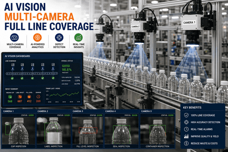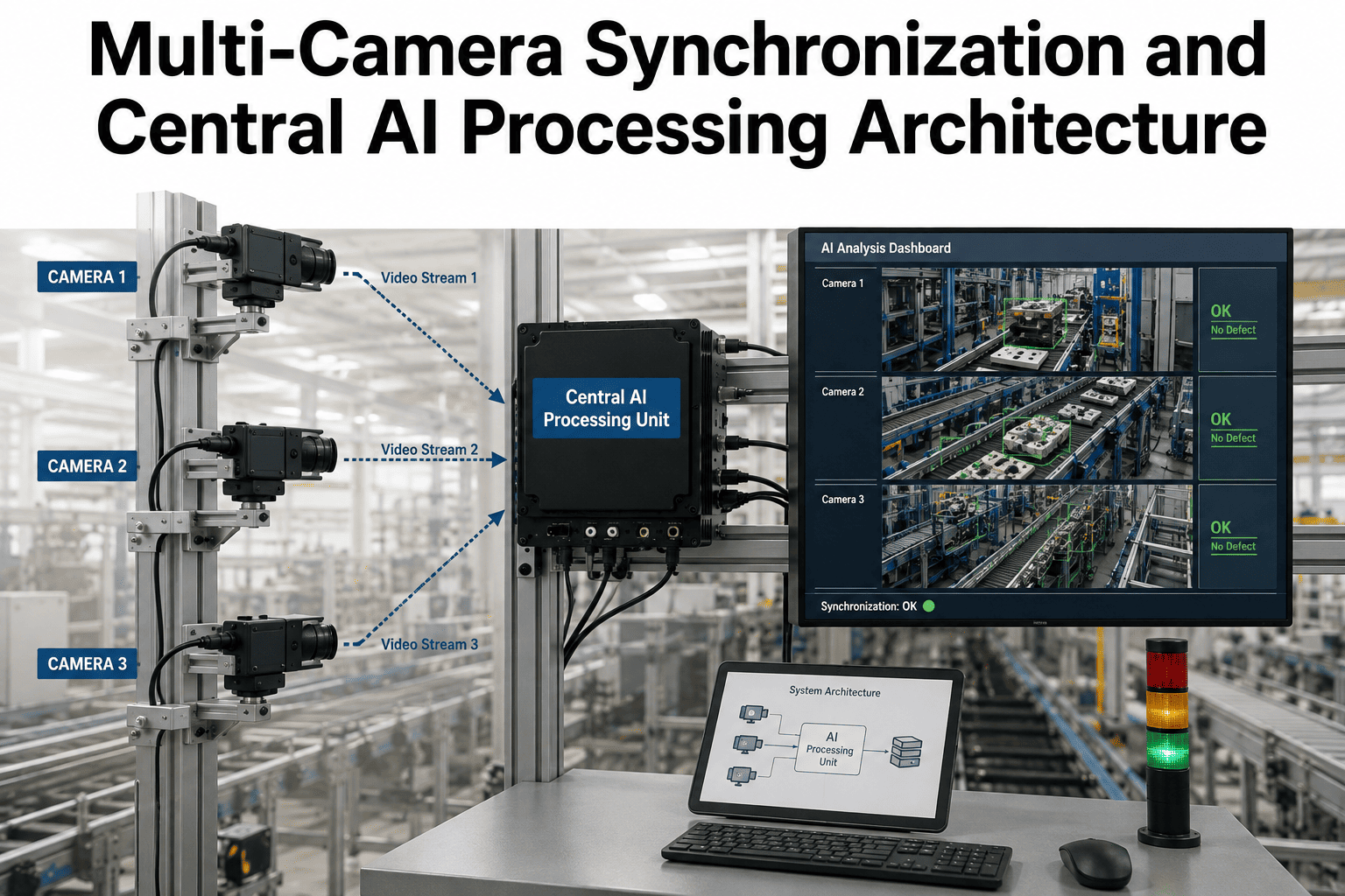
A single inspection camera is an engineering exercise. Fifty cameras running against one process, one clock, and one verdict is an architecture problem — and it is where most industrial vision projects quietly stall. Frames arrive milliseconds apart, GPUs sit idle while others choke, and one failed edge box silently drops a station from coverage for an entire shift. Getting 10, 50, or 100+ cameras to behave as one synchronized instrument requires deliberate decisions about timing, transport, batching, and failover. If you are sizing that architecture right now, book a demo and we will map your camera count against real GPU server configurations.
Synchronize 100+ Cameras to a Single AI Brain Without Dropping a Frame, a Verdict, or a Shift
A complete architecture reference for centralized multi-camera vision: how to lock every sensor to a common clock, size the NVIDIA GPU server behind them, balance load across streams, and build the redundancy that mission-critical inspection actually demands.
The Camera Was Never the Hard Part — Coordinating Fifty of Them Is
Almost every industrial vision deployment starts the same way. One camera, one station, one model, one clear win. The pilot works, the plant sees the defect catch rate, and leadership asks the obvious question: can we do this everywhere? That is the moment the project changes character entirely. Scaling from one camera to fifty is not a procurement exercise where you multiply the bill of materials by fifty. It is an architecture problem in which timing, bandwidth, compute scheduling, and failure behavior all become first-order design constraints that simply did not exist at the single-camera scale.
The failure mode is predictable. Teams buy fifty cameras and fifty small edge computers, deploy them station by station, and discover eighteen months later that they are maintaining fifty independent software environments, fifty model versions that have drifted apart, fifty sets of logs that cannot be correlated, and fifty single points of failure that nobody is monitoring. Meanwhile the analytics team cannot answer a basic question — did the defect at Station 7 correlate with the temperature excursion seen by Station 3 four seconds earlier — because no two devices agree on what time it was.
Centralized processing inverts every one of those problems. One server, one model registry, one clock domain, one place to patch, one place to monitor, and one place to correlate. The trade-off is that the central architecture has to be engineered properly from day one, because everything now depends on it. That is what the rest of this guide covers: the specific decisions that make a centralized multi-camera vision system reliable enough to run a production line on.
Distributed Edge Boxes Versus a Central AI Server — Where Each Model Breaks
Both architectures are legitimate, and the honest answer is that the right choice depends on camera count, latency requirement, and network topology. What follows is not a sales argument for one approach but the operational reality of each once you pass roughly a dozen cameras and start living with the system across shifts, model updates, and hardware failures.
Clock Drift Between Nodes
Each box keeps its own time. Without a disciplined PTP domain, timestamps diverge by tens of milliseconds, making cross-station correlation and root-cause analysis effectively impossible.
Model Version Fragmentation
A retrained model has to be pushed to every node individually. In practice, some nodes lag by weeks, so two stations inspecting the same defect apply different acceptance thresholds.
Stranded Compute Capacity
Every node is sized for its own peak. A station running at 20 percent utilization cannot lend headroom to the station next to it that is saturated during changeover.
Distributed Failure Surface
Fifty boxes in cabinets across a plant means fifty thermal environments, fifty power feeds, and fifty devices that can fail quietly without anyone noticing until a quality escape surfaces downstream.
Single Clock Domain
Every frame carries a timestamp from the same grandmaster clock, so frames from different cameras can be joined, replayed, and analyzed as one coherent event stream.
One Model Registry
Deploy a retrained model once and every camera in the plant inherits it in the same instant, with a version history that ties every historical verdict to the exact model that produced it.
Pooled, Load-Balanced Compute
Batched inference lets a saturated station borrow GPU headroom from idle ones, which is why a central server usually serves more cameras than the sum of equivalent edge nodes.
Concentrated, Monitorable Failure Domain
One rack to instrument, cool, and protect on UPS, with N+1 standby that can assume the full camera load automatically rather than fifty independent devices to babysit.
The concentration of risk in a central architecture is real and should not be minimized. The answer is not to avoid centralizing but to engineer redundancy deliberately, which is covered in detail further down this page. A single well-instrumented server with a hot standby is far easier to make genuinely reliable than fifty unmonitored boxes distributed across a plant floor.
Four Layers of Timing, and What Each One Actually Buys You
Synchronization is not a single setting. It is a stack, and each layer delivers a different order of accuracy at a different cost and cabling burden. Choosing the wrong layer is expensive in both directions: over-engineering a general surface-inspection application with hardware trigger wiring wastes budget, while under-engineering a high-speed multi-view measurement application with software triggers produces data that quietly cannot be trusted.
Hardware Trigger Distribution
A dedicated trigger line from an encoder, PLC, or trigger box fires every camera on the same physical edge. Highest determinism available, and still the reference standard for high-speed measurement and multi-view metrology.
PTP With Scheduled Action Commands
Cameras negotiate a master clock over the network and execute a captured action at a specified future timestamp, restoring real-time behavior over standard Ethernet without physical trigger lines. This is the sweet spot for most plant-scale deployments.
PTP Timestamping Without Scheduled Triggers
Cameras free-run but stamp every frame against a shared clock, so the server can align streams after capture. Adequate for correlation, analytics, and event reconstruction, but not for simultaneous exposure of a moving object.
Software Trigger and Free-Run
The host sends a capture command over the network to each camera in turn. Network propagation and firmware processing delays make true simultaneity impossible, which is exactly the gap the PTP-plus-action-command combination was created to close.
| Sync Method | Typical Accuracy | Cabling Required | Best Fit Application |
|---|---|---|---|
| Hardware trigger line | Nanosecond class | Dedicated trigger cable per camera | High-speed metrology, multi-view 3D reconstruction |
| PTP with scheduled action command | Sub-microsecond to low microsecond | Standard Ethernet, PTP-aware switches | Plant-wide inspection, conveyor multi-angle capture |
| PTP timestamp only | Post-capture alignment | Standard Ethernet | Analytics, event correlation, forensic replay |
| Software trigger | Millisecond class, variable | Standard Ethernet | Static inspection, low-speed stations only |
| Free-run capture | No guaranteed relationship | Standard Ethernet | Continuous monitoring where timing is not material |
One practical note that trips up more deployments than any other: PTP accuracy is a property of the network, not just the cameras. Consumer-grade unmanaged switches introduce variable queuing delay that destroys the precision the protocol is capable of. Boundary-clock or transparent-clock switches, a disciplined grandmaster, and a camera VLAN free of unrelated traffic are what turn a theoretical microsecond into a delivered microsecond.
Not Sure Which Sync Layer Your Application Actually Requires?
Over-engineering timing wastes budget and cabling. Under-engineering it produces measurement data your quality team cannot defend during an audit. Walk your line layout, camera count, and line speed through with our architecture team and get a specific recommendation on sync layer, switch topology, and GPU server sizing before you commit to hardware.
How Much GPU Server You Need for 10, 50, or 100+ Cameras
Stream density on a GPU is not a single number, and any vendor quoting one without asking about your resolution, frame rate, and model architecture is guessing. Three variables dominate. Decode capacity is handled by dedicated hardware decoder units that are separate from the compute cores, so decode and inference do not directly compete. Inference throughput depends on model size and batch efficiency. Memory bandwidth and pipeline overhead — scaling, color conversion, dewarping, and drawing outputs — often become the real ceiling well before raw compute does.
The single most common sizing mistake is treating the camera count as the requirement. It is not. The requirement is aggregate pixel throughput multiplied by model complexity, and a dozen high-resolution cameras inspecting fine surface defects at high frame rate can be a heavier workload than sixty standard-resolution cameras doing presence-absence checks. Always size against pixels per second and model cost, then validate with a benchmark on your actual images before the purchase order goes out.
The Ingest Math Everyone Skips Until the Network Falls Over
Camera bandwidth is arithmetic, not opinion, and it is worth doing on paper before a single cable is pulled. Uncompressed frame payload is width multiplied by height multiplied by bytes per pixel multiplied by frames per second. A single gigabit link tops out at roughly 125 megabytes per second of usable payload, which is why oversubscribing a switch port or a server NIC produces dropped packets that look exactly like a camera fault and are diagnosed as one for weeks.
| Configuration | Per-Camera Payload | 25 Cameras | Recommended Server Ingest |
|---|---|---|---|
| 2MP mono at 30 fps | Approximately 60 MB/s | Approximately 1.5 GB/s | Dual 10GbE minimum, 25GbE preferred |
| 5MP color at 20 fps | Approximately 300 MB/s | Exceeds practical single-fabric ingest | Compression or on-camera ROI required |
| 1080p H.265 stream at 30 fps | Approximately 0.5 to 1 MB/s | Approximately 25 MB/s | Single 10GbE comfortably sufficient |
| 4K H.265 stream at 15 fps | Approximately 1.5 to 3 MB/s | Approximately 75 MB/s | 10GbE with headroom for burst and archive writes |
The table makes the central architectural fork obvious. Raw uncompressed GigE Vision streams give you pristine pixels for measurement-grade inspection but consume bandwidth aggressively, which caps camera count per fabric segment. Compressed streams decoded on the server's hardware decoder units scale to far higher camera counts at the cost of some compression artifact, which is entirely acceptable for detection and classification work and unacceptable for sub-pixel metrology. Most real plants run both: a small raw-stream measurement cluster and a large compressed-stream monitoring and detection estate, converging on the same server and the same model registry.
Three practical mitigations keep bandwidth manageable without abandoning image quality. Region-of-interest cropping on the camera transmits only the pixels that matter, often cutting payload by seventy percent or more. Triggered burst capture sends frames only when a part is actually present rather than streaming continuously. Per-camera bandwidth throttling prevents any single sensor from starving its neighbors during a burst. Applied together, these three routinely double or triple the camera count a given fabric can support.
Where the Milliseconds Actually Go Between Exposure and Reject Signal
When a line runs at a fixed rate and a reject mechanism sits a fixed distance downstream, the vision system has a hard, non-negotiable latency budget. Missing it does not degrade quality gracefully — it means bad parts pass the ejector before the verdict arrives. Understanding where the time is spent is what lets you engineer against the budget instead of hoping the system is fast enough.
Exposure and Readout
Fixed by sensor and lighting design. Global shutter sensors avoid the motion skew that makes rolling shutter unusable on fast lines, which is a sensor selection decision, not a software one.
Network Transport
The most variable segment and the one most improved by architecture. Congestion, unmanaged switch queuing, and shared VLANs introduce jitter that shows up as unpredictable verdict timing.
Decode and Preprocess
Hardware decoder units handle compressed streams without touching compute cores, but scaling, color conversion, and dewarping run on the GPU and consume real budget at high camera counts.
Inference
Usually the largest single block. Batching improves throughput substantially but adds queue wait, so the batch size that maximizes frames per second is rarely the one that minimizes worst-case latency.
Verdict Assembly
Post-processing, threshold application, multi-camera fusion where several views vote on one part, and writing the inspection record to the historian for later audit and traceability.
Actuation Signal
Delivery of the pass or fail signal to the PLC or reject mechanism over the control network, including whatever scan-cycle delay the controller itself contributes to the loop.
The critical insight for centralized architectures is that you must design against worst-case latency, not average. A system with a five millisecond average and a ninety-nine millisecond tail will fail an audit and let bad parts through, even though its dashboard looks healthy. That means bounded queue depths, per-stream latency ceilings, priority scheduling that lets a safety-critical station preempt a monitoring station, and continuous monitoring of the ninety-ninth percentile rather than the mean.
Four Tiers of Resilience, Matched to What an Outage Actually Costs You
Centralizing processing concentrates risk, and pretending otherwise is how vision projects lose credibility with operations leadership. The correct response is to size redundancy against consequence. A monitoring camera going dark for an hour is an inconvenience. A release-gating inspection station going dark for an hour may stop the line or block product from shipping. These should not receive the same architecture, and paying for the highest tier everywhere is as much a design failure as paying for none of it.
Buffer and Replay
Cameras or an edge collector buffer frames locally when the server is unreachable, then replay on recovery. Verdicts arrive late but no inspection record is lost, which preserves traceability even through a short outage.
Redundant Network Paths
Ring or dual-homed topology with rapid reconvergence so a single cable pull, switch failure, or accidental disconnection during maintenance does not remove a station group from coverage.
N+1 Warm Standby Server
A second server holds current models loaded and assumes the full camera load on health-check failure. Recovery measured in seconds, with stream assignment handled automatically rather than by a call to the integrator.
Active-Active With Priority Shedding
Two servers share the camera load in normal operation. If one fails, the survivor keeps every release-gating station running at full rate and gracefully sheds monitoring streams until capacity is restored.
Health Telemetry on Every Stream
Per-camera frame rate, dropped packet count, PTP offset, and inference latency monitored continuously, so a degrading camera is caught as a trend rather than discovered during a quality escape investigation.
Defined Degraded-Mode Behavior
Written, tested rules for what the line does when vision is unavailable — hold, pass with manual check, or stop — agreed with quality before deployment rather than improvised during the first incident.
Test the failover. A standby server that has never been proven under a real cutover is a document, not a control. The teams that get this right schedule a deliberate failover during planned downtime at least twice a year, measure the actual recovery time, and confirm that every camera reattaches to the surviving node with the correct model version loaded.
From Site Survey to Live Production in Six to Twelve Weeks
Centralized vision architecture sounds like a long infrastructure program, and traditionally it was. The reason it no longer has to be is that the hardware arrives pre-configured. iFactory ships a turnkey NVIDIA AI server racked, imaged, and benchmarked against your camera specification, so site work is cabling, calibration, and validation rather than months of platform engineering. Below is the sequence that gets a plant from survey to production verdicts.
Survey, Sizing, and Network Design
Camera count, resolution, and frame rate captured per station. Aggregate bandwidth and pixel throughput calculated. Sync layer selected per application. Switch topology, VLAN plan, and PTP grandmaster placement designed. Server configuration finalized against benchmarked model cost on your actual sample images rather than a generic reference dataset.
Install, Synchronize, and Calibrate
Pre-configured server racked and connected. Cameras mounted, lit, and focused. PTP domain established and offset verified across every sensor. Streams brought online in station groups, with baseline images collected under production lighting and line speed to tune models against real conditions instead of laboratory samples.
Validate, Integrate, and Hand Over
Shadow-mode running alongside existing inspection to compare verdicts before anything gates production. PLC integration and reject-signal timing validated against the latency budget. Failover tested under load. Operator training completed, degraded-mode rules signed off with quality, and the system transitioned to live gating with full traceability.
That conversation is only possible because every camera shares one clock, one model registry, and one inspection record. On a distributed architecture with independent nodes and drifting timestamps, correlating a defect to a tooling change six minutes earlier is a manual investigation spanning several log files. On a centralized architecture it is a question with an immediate answer.
Six Design Errors That Surface Only After Go-Live
Every one of the following has been diagnosed as a camera fault at least once before somebody traced it back to architecture. They are cheap to prevent during design and expensive to fix after cabinets are populated and cable trays are full.
Unmanaged Switches in a PTP Domain
Variable queuing delay in consumer-grade switching hardware destroys the timing precision the protocol can deliver. The system appears synchronized in testing with light traffic and drifts unpredictably under full production load.
Sizing by Camera Count Alone
Twelve high-resolution cameras running a heavy segmentation model can outweigh sixty cameras doing simple presence checks. Size against pixels per second and model cost, then validate with a benchmark on your own images.
Cameras Sharing a Business VLAN
Vision traffic on the same segment as backups, file transfers, and general plant IT produces intermittent frame drops that correlate with nothing an operator can see, and take weeks to diagnose without dedicated segmentation.
Tuning Batch Size for Throughput Only
Large batches raise aggregate frames per second while pushing worst-case latency past the reject window. Tune for the ninety-ninth percentile latency the line actually requires, not for the headline throughput number.
No Archive Retention Policy
Storing every frame from every camera indefinitely fills any volume eventually. Define retention per station criticality up front, keeping failures and a sampled pass set rather than the entire raw stream forever.
Untested Failover
A standby server that has never handled a real cutover is documentation, not resilience. Schedule deliberate failover during planned downtime and measure the true recovery time with every camera reattaching correctly.
Sixty-Four Cameras Across Three Lines on One Central Architecture
Consider a mid-size manufacturing plant with three assembly lines and sixty-four inspection points. Twelve of those points are release-gating measurement stations requiring raw uncompressed imagery and tight simultaneity between paired views. The remaining fifty-two are detection and monitoring stations checking presence, orientation, surface condition, and label accuracy, where compressed streams are perfectly adequate.
Under a distributed plan, this becomes sixty-four edge devices in sixty-four cabinets, each with its own operating system, driver stack, model copy, and thermal environment. Assume a conservative annual failure rate and the plant can expect several silent device failures per year, each one removing a station from coverage until somebody notices. Model updates require sixty-four separate deployments. Correlating an event across lines is a manual exercise across sixty-four uncoordinated log files.
Under the centralized plan, the twelve measurement stations run on a raw-stream segment with hardware trigger distribution for the paired views and dedicated fabric bandwidth. The fifty-two detection stations run compressed streams over a segmented, PTP-disciplined vision VLAN into the same server pair. Two GPU servers operate active-active, with the twelve gating stations designated priority streams that never shed. A tooling change, a lighting degradation, or a supplier material shift becomes visible as a pattern across stations within minutes rather than a quality escape found downstream.
The operational difference is not primarily cost, although consolidating sixty-four devices into two servers does change the maintenance burden materially. The difference is that the plant now has one coherent inspection record with a single time base across every line, which is what makes cross-station analytics, model improvement, and audit defensibility possible at all. That capability does not exist in the distributed version at any price.
What Engineering Teams Ask Before Committing to a Central Architecture
Get Your Multi-Camera Architecture Sized Before You Buy the Hardware
Bring your camera count, resolution, line speed, and latency requirement. We will return a specific architecture — sync layer, switch topology, GPU server configuration, bandwidth plan, and redundancy tier — benchmarked against your own sample images rather than a generic reference. Pre-configured NVIDIA AI servers ship racked and ready, with a six to twelve week path from survey to live production verdicts across every camera in the plant.