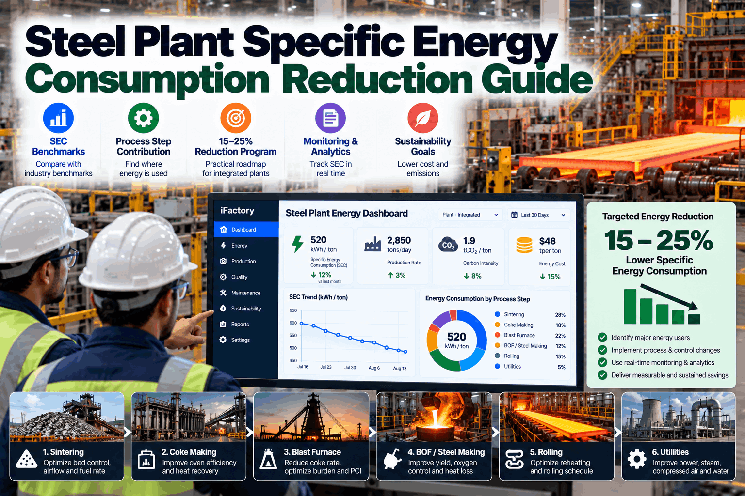
A steel plant historian that stores 400,000 tags at one-second resolution and cannot answer the question "what was the specific energy consumption of the EAF in GJ per tonne of liquid steel last shift, corrected for scrap grade mix" is not an analytics asset — it is an archive. The difference between a historian configured for compliance logging and one configured for energy analytics is not the volume of data it holds. It is the tag naming convention that makes process context machine-readable, the compression settings that preserve the precision energy calculations require, the aggregation architecture that lets a query return a GJ/t trend across six months in under three seconds, and the data model that links every energy reading to the production event it belongs to. Most steel plant historians were designed by control engineers to support operators. Reconfiguring them to support energy analytics — without disrupting the operational layer — is a specific engineering problem with a specific set of answers. iFactory Steel Energy Analytics is built on that architecture — historian-native, GJ/t and kWh/t benchmarked, live across every energy centre.
iFactory Steel Energy Analytics — Historian Architecture Guide
Steel Plant Energy Data Historian Design for Analytics
Tag naming conventions, time-series architecture, compression settings, and query patterns that turn a steel plant historian from a compliance archive into a live GJ/t and kWh/t analytics platform.
400K+
tags typical in a large integrated steel plant historian
<3 sec
target query return for a 6-month GJ/t trend — correctly indexed
GJ/t & kWh/t
specific energy — the KPI historians are rarely built to serve
Historian-native
PI, AVEVA, Aspen — no data lake required to get analytics
Why Most Steel Plant Historians Fail at Energy Analytics
The historian is already collecting the data. The EAF power meter is already writing to a tag. The gas flow transmitter has been logging since commissioning. The problem is not data availability — it is data accessibility. These are the six configuration failures that make an energy-rich historian produce energy-poor analytics.
01
No production context linkage
Energy tags store kWh readings with timestamps. Heat numbers, cast sequences, and shift codes live in the MES or ERP. Without a join key embedded in the historian or the data model, every GJ/t calculation requires a manual merge that nobody does every shift.
02
Compression destroys precision
Exception reporting compression — the default in PI and AVEVA — is tuned for trending, not for energy integration. A deadband of 0.5% on a 40 MW EAF power tag can introduce a 2–4% error into a heat energy calculation. For GJ/t benchmarking, that is the entire improvement target.
03
Tag naming carries no semantic meaning
Tags named PLC04.AI_0142 or EAF1_KW_001 cannot be filtered, grouped, or queried by process area, energy type, or production unit without a separate lookup table that is never maintained after commissioning.
04
No aggregated energy tags
Querying raw one-second power readings to compute a shift energy total across 40 sub-metered circuits is a calculation that takes minutes and locks the historian server. Without pre-aggregated hourly and shift energy tags, ad-hoc analytics stalls the operational layer.
05
Mixed engineering units across areas
Electrical energy in MWh, gas in Nm³, steam in tonnes, oxygen in Nm³/hr — with conversion factors to GJ embedded in spreadsheets held by three different engineers. Any cross-energy-type comparison requires a manual conversion step that varies by analyst.
06
No state or mode tagging
An EAF drawing 38 MW during a meltdown and drawing 8 MW during a tap delay look identical in the energy data without a mode tag. Specific energy calculated without filtering to active production periods inflates the GJ/t figure by 15–30% on a typical EAF heat cycle.
Tag Naming Convention — The Foundation of Queryable Energy Data
A tag naming standard is the single highest-leverage investment in steel plant historian analytics. It is not glamorous and it does not require new hardware — but without it, every query requires a lookup table, every dashboard requires manual curation, and every new analyst starts from scratch. The convention below is structured for a steel plant energy historian and follows a hierarchy that supports filtering at every level.
Recommended Tag Name Structure
SITE
Plant / site code
BSP1
.
AREA
Process area
EAF · BOF · CCM · RHF · HRM
.
UNIT
Equipment unit number
01 · 02 · 03
.
ETYPE
Energy type
ELEC · GAS · O2 · N2 · STM
.
MEAS
Measurement type
PWR · FLOW · ENRG · CUMU
.
UOM
Unit of measure
MW · GJ · NM3H · T
Example Tags — Correctly Named
BSP1.EAF.01.ELEC.PWR.MW
EAF 1 — active electrical power draw in MW
BSP1.EAF.01.ELEC.ENRG.GJ
EAF 1 — cumulative electrical energy in GJ (heat-reset)
BSP1.EAF.01.GAS.FLOW.NM3H
EAF 1 — natural gas flow rate in Nm³/hr
BSP1.RHF.01.GAS.ENRG.GJ
Reheating furnace 1 — cumulative gas energy in GJ (shift-reset)
BSP1.EAF.01.MODE.STATE.ENUM
EAF 1 — heat mode state (0=idle, 1=melt, 2=refine, 3=tap, 4=delay)
BSP1.EAF.01.PROD.HEAT.ID
EAF 1 — current heat number (string tag, links to MES)
Historian Architecture Layers — Raw Data to Analytics-Ready
A steel plant energy historian built for analytics operates in three distinct data layers. Conflating them — writing analytics calculations directly against raw one-second tags — is what makes steel plant historian queries slow, brittle, and impossible to maintain when the instrument configuration changes.
Layer 1
Raw Instrument Layer
One-second to one-minute resolution. Direct from PLC/DCS via OPC-UA or Modbus. Compression settings tuned per tag type — tight deadband for energy meters (≤0.1%), wider for temperature trends (±1°C acceptable). Never queried directly by analytics layer.
↓
Layer 2
Calculated & Aggregated Tag Layer
Derived tags calculated in the historian (PI Analytics / AVEVA Calculation Engine) or in a lightweight edge calculation service. Energy totals per heat, per shift, and per hour. Mode-filtered calculations that exclude delay states. Specific energy in GJ/t when linked to production weight tags.
↓
Layer 3
Analytics & Benchmark Layer
Pre-aggregated hourly and shift summaries stored as historian tags or in a connected time-series database (InfluxDB, TimescaleDB) for cross-area queries. Benchmark comparisons against rolling 30/90-day baselines. KPI dashboard tags consumed by iFactory or PI Vision without real-time computation.
Compression Settings — Where GJ/t Accuracy Is Won or Lost
Exception reporting compression — the default setting in every major historian — stores a new value only when the signal changes by more than a defined deadband. For trend visualisation, this is efficient and accurate enough. For energy integration over a heat cycle, a poorly set deadband on a high-power tag introduces a systematic error that can dwarf the efficiency improvement being measured. These are the compression settings that matter for energy analytics in a steel plant.
Tag Category
Example
Recommended Deadband
Max Interval
Why It Matters
CriticalEAF / LF power meter
BSP1.EAF.01.ELEC.PWR.MW
≤0.05% of span
5 seconds
Integration error compounds over a 60-min heat — 0.5% deadband = 2–4% GJ error
CriticalGas flow meter
BSP1.RHF.01.GAS.FLOW.NM3H
≤0.1% of span
10 seconds
RHF gas consumption varies slowly — high deadband misses the slow drift that is the entire optimisation target
ImportantOxygen / nitrogen flow
BSP1.EAF.01.O2.FLOW.NM3H
≤0.2% of span
10 seconds
O₂ lance flow changes fast during blowing — coarse deadband misses the step changes that drive melt energy calculations
ImportantSteam flow meter
BSP1.STM.MAIN.FLOW.TH
≤0.2% of span
30 seconds
Steam is slow-moving — 30s max interval prevents data gaps at constant load, but tighter deadband needed for waste heat recovery quantification
StandardProcess temperature
BSP1.RHF.01.TEMP.Z3.DEG
±1°C or 0.5%
60 seconds
Used for process monitoring, not energy integration — standard compression sufficient for trending and alarm management
StandardUtility pressure
BSP1.COMP.AIR.PRESS.BAR
±0.5% of span
60 seconds
Trend monitoring — tighter compression not justified unless compressed air energy metering is part of the analytics scope
Query Patterns — The Four Calculations Steel Energy Analytics Runs Every Day
A steel plant energy historian configured correctly supports four core query patterns that together constitute the daily energy analytics workflow. Each one has a specific data requirement that flows back to the architecture and tag naming decisions above.
Q1
Heat-level specific energy — EAF
Returns GJ/t of liquid steel for each heat over a selected period, mode-filtered to exclude delays. The core EAF benchmarking calculation.
Data requirements
Heat start/end timestamps — from MODE.STATE.ENUM tag or MES event feed
Electrical energy per heat — integrated from ELEC.PWR.MW over heat window, mode=1,2 only
Gas + oxygen energy per heat — flow integrated and converted to GJ (9.5 MJ/Nm³ gas, 0.5 MJ/Nm³ O₂ credit)
Liquid steel weight — from PROD.HEAT.WT_LS.T tag or MES join on PROD.HEAT.ID
Output: GJ/t per heat — trended, benchmarked against 30-day rolling average
Q2
Shift energy balance — plant-wide
Returns total energy by type (electrical, gas, oxygen, steam) per process area per shift. Cross-area balance check — grid import vs sum of area submeters.
Data requirements
Shift boundary timestamps — from production schedule or fixed shift pattern tag
Area energy totals — pre-aggregated ENRG_SHIFT.GJ tags per area (Layer 2)
Utility metering — grid import MWh, gas Nm³, O₂ Nm³ — shift-accumulated
Unit conversion factors — standardised to GJ: 1 MWh = 3.6 GJ, gas at site-specific GCV
Output: GJ by energy type per area per shift — balance check flags measurement gaps
Q3
Reheating furnace efficiency — GJ/t rolled
Returns GJ per tonne of hot-rolled steel for the RHF, normalised for slab entry temperature and target exit temperature. The primary rolling mill energy KPI.
Data requirements
Gas consumption per campaign — GAS.ENRG.GJ accumulated over slab sequence
Slab weight throughput — PROD.RHF.WT_SLAB.T per campaign from scale or MES
Slab entry temperature — TEMP.SLAB_IN.DEG for cold vs hot charge normalisation
Furnace idle energy — MODE.STATE.ENUM to exclude soak-hold and idle periods from denominator
Output: GJ/t rolled — temperature-normalised — idle-excluded baseline trend
Q4
Baseline deviation alert — any energy centre
Returns real-time deviation of current-shift specific energy vs 30-day rolling baseline for each energy centre. The primary operational alert that drives same-shift intervention.
Data requirements
Current shift GJ/t — from Layer 2 calculated tag, updated every completed heat or hour
30-day rolling baseline GJ/t — pre-computed Layer 3 tag, updated daily
Deviation % tag — KPI.DEVIATION_PCT calculated in historian or iFactory analytics layer
Alert threshold — configurable per energy centre (typical: +5% for EAF, +8% for RHF)
Output: % deviation from baseline — live — alert fired to shift manager when threshold breached
GJ/t and kWh/t Benchmarks — Steel Process Energy Reference
Specific energy benchmarks give the historian architecture its purpose — they are the targets that calculated tags are measured against. These are the industry reference ranges for each major steel plant process, against which iFactory's analytics layer benchmarks live historian data. The gap between actual and benchmark is where the energy cost recovery lives.
Process
Best-in-class
Fleet average
Laggard
Primary energy driver
EAF — liquid steel
1.8–2.2 GJ/t
2.4–2.8 GJ/t
3.0–3.5 GJ/t
Scrap grade mix, tap-to-tap time, O₂ use
BOF — liquid steel
0.5–0.9 GJ/t
1.0–1.4 GJ/t
1.5–2.0 GJ/t
Hot metal ratio, scrap charge temp, O₂ lance practice
Ladle furnace (LF)
0.06–0.10 GJ/t
0.12–0.18 GJ/t
0.20–0.30 GJ/t
Tap temperature precision, lid practice, holding time
Reheating furnace (RHF)
1.0–1.3 GJ/t
1.5–2.0 GJ/t
2.2–2.8 GJ/t
Hot charging ratio, idle soak time, excess air, recuperation
Hot rolling mill
40–60 kWh/t
70–100 kWh/t
110–140 kWh/t
Pass schedule efficiency, roll force, cobble rate, idle power
Cold rolling mill
50–80 kWh/t
90–130 kWh/t
140–180 kWh/t
Reduction schedule, roll force control, annealing cycle optimisation
Continuous caster (CCM)
8–12 kWh/t
14–20 kWh/t
22–30 kWh/t
Cooling water pump efficiency, dummy bar energy, heat sequence length
Compressed air (plant)
0.08–0.11 kWh/Nm³
0.13–0.18 kWh/Nm³
0.20–0.28 kWh/Nm³
Compressor efficiency, distribution pressure, leak rate, demand management
Want to see where your process areas sit against these benchmarks using your own historian data? Book a demo — connect your PI or AVEVA instance and we'll run the GJ/t calculations live on your data in the first session.
Historian Platform Support — PI, AVEVA, Aspen and Beyond
The architecture principles above apply regardless of historian platform. The implementation details — API endpoint, calculation engine syntax, tag attribute names — differ by platform. These are the four historian platforms most common in steel plant environments and what iFactory connects to natively in each case.
How iFactory Connects to Your Historian — From Tag Audit to Live GJ/t
The path from a steel plant historian in its current state to a live GJ/t analytics dashboard is five engineering steps. Each one is where iFactory replaces a configuration assumption with a validated, tested, and documented data pipeline.
01
Tag Audit
iFactory scans the historian tag list, identifies energy-relevant tags by keyword and unit-of-measure, flags compression settings that introduce integration error, and maps existing tags to the recommended naming convention. Output: a tag audit report with remediation priority.
02
Layer 2 Build
Calculated tags built in the historian's native calculation engine — heat energy totals, shift aggregations, mode-filtered specific energy. Production context linked via MES event feed or PI AF element. No external computation required for operational queries.
03
Benchmark Baseline
30-day and 90-day rolling baseline GJ/t calculated per energy centre from historian history. Baseline tags written back to historian so deviation detection runs natively. Process-normalised baselines where scrap grade or hot charge ratio varies significantly.
04
iFactory Connection
iFactory connects to Layer 2 and Layer 3 tags via PI Web API, REST, or OPC-UA. Live GJ/t dashboard populated from pre-calculated tags — query response under 3 seconds regardless of historian scale. No raw tag queries from the analytics layer.
05
Live Deviation Alerts
Deviation % tags monitored in real time. Alert fired to shift energy manager when any energy centre exceeds baseline threshold — with energy centre, current GJ/t, baseline GJ/t, and estimated cost of deviation per remaining shift hours. Same-shift intervention enabled.
What a Correctly Architected Steel Energy Historian Delivers
The return on historian architecture investment in a steel plant is measured in the same currency as production — GJ/t reduced, cost per tonne lowered, and energy deviations caught in the same shift rather than in the next month's management report. These are the outcomes steel plants achieve when the historian is configured for analytics rather than just logging.
<3 sec
Query response
6-month GJ/t trend — pre-aggregated Layer 3 architecture
Heat-level
GJ/t resolution
every heat benchmarked — not a shift average or monthly total
Same shift
Deviation detection
baseline alert fires before the deviation compounds across a campaign
Historian-native
No data lake required
PI, AVEVA, Aspen — analytics run from existing infrastructure
Frequently Asked Questions
Do we need to re-tag our existing historian to use iFactory?
Not immediately. iFactory connects to existing tag names and maps them to the recommended naming convention in the analytics layer — so your existing PI or AVEVA installation continues to work for operators and control engineers exactly as it does today. The naming convention remediation is a phased programme applied to new tags and revised during instrument or control system upgrades. For the initial analytics deployment, we work with what exists and build the naming layer in iFactory's tag mapping configuration. The historian-level rename is a medium-term data governance programme, not a prerequisite for going live.
How do we handle the production context link — heat numbers, shift codes — if they're in the MES and not the historian?
There are three approaches, in order of preference. First: write heat number as a string tag to the historian from the MES at heat start and end — this makes every energy query self-contained within the historian. Second: use PI AF element templates that pull heat attributes from the MES via event frames — the historian data and the MES data are linked in the asset model without tag writing. Third: maintain a lightweight join table in iFactory that maps heat number to timestamp windows — extracted from the MES on a scheduled basis. The first approach is the cleanest for analytics. The third is the fastest to implement where MES access is restricted.
How do we handle multi-energy GJ/t calculations where the conversion factors differ by fuel grade?
Calorific value variation — particularly for BFG, COG, and mixed gas streams — is handled by linking a calorific value tag to the energy calculation. In PI Analytics, the calculated tag for gas energy in GJ reads the flow tag (Nm³/hr) and multiplies by a GCV tag that is updated from the laboratory analysis on the shift schedule — typically once per shift or on demand. The GCV tag is written manually or fed from the gas analyser. This approach means the GJ/t figure reflects the actual fuel quality delivered in each heat, not a fixed assumed GCV that drifts from reality as blast furnace conditions change.
What does the tag audit process involve and how long does it take?
The tag audit reads the historian's tag list — typically exported as a CSV or accessed via API — and applies a classification algorithm that identifies energy-relevant tags by unit of measure, description keywords, and source PLC/DCS node. For a 400,000-tag historian, this classification runs in under an hour. The output is a prioritised list of energy tags with their current compression settings, a flag for any settings that introduce integration error above a defined threshold, and a proposed mapping to the naming convention. A full audit report covering electrical, gas, oxygen, steam, and water energy tags across all major process areas typically takes one to two weeks including review with the plant's instrumentation and control team.
Can we start with one process area before committing to the full plant architecture?
Yes — and for a steel plant, the EAF is almost always the right starting point. It is the highest single energy consumer in an EAF-based plant, has the clearest heat-level production event boundary for GJ/t calculation, and is where the gap between actual and benchmark specific energy is typically largest and most directly actionable. An EAF pilot covers the tag audit for the EAF energy circuits, Layer 2 calculated tags for heat energy and specific energy, baseline GJ/t from 90 days of history, and a live deviation alert on the iFactory dashboard. Book a demo with read access to your PI or AVEVA instance and we'll run the GJ/t calculation on your data in the first session.
Your historian already has the data. Build the architecture to use it.
See Live GJ/t Analytics Running on Your Steel Plant Historian
Bring read access to your PI, AVEVA, or Aspen historian and your EAF or RHF energy tag list. We'll run the tag audit, calculate heat-level GJ/t from your historical data, and show the deviation from your 30-day baseline — in the first session, on your own data.
PI / AVEVA
native connect
Same shift
deviation alert