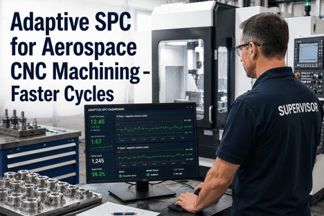
Adaptive SPC for Aerospace CNC Machining – Faster Cycles
By Grace on June 9, 2026
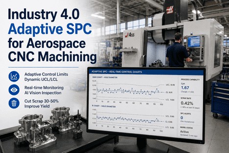
The control limits on the SPC chart were set during process qualification 16 months ago. At the time, the CpK was 1.67, the machine was new, and the tooling specification matched the production intent exactly. Today, the coolant concentration is different, the material batch has a slightly different heat treat response, and the fixture has accumulated 12,000 part cycles of wear. The control limits have not changed. Every shift, the operator sees points that fall outside the old limits — not because the process is defective, but because the limits no longer describe the process that exists on the floor. Some of these signals are false alarms. Some are real. The operator cannot distinguish between them because the chart does not either. The result is a control system that operators learn to ignore — because a chart that cries wolf too often is a chart that nobody trusts when the wolf actually arrives. Adaptive control limits solve this by recalculating UCL and LCL dynamically against current process behaviour, so the limits always reflect the real process — not the one that existed during a study conducted years ago.
The Control Limits on Your SPC Chart Describe the Process That Existed 16 Months Ago. Adaptive Limits Describe the One Running Right Now.
iFactory's adaptive control limit platform replaces fixed UCL/LCL with self-adjusting statistical models that tighten during stable periods and widen during natural process variation — eliminating false alarms while catching real drift earlier than static charts ever could.
False alarm reduction achieved when aerospace CNC cells replace static control limits with adaptive limits that adjust UCL and LCL dynamically to current process behaviour
3–5x
Faster detection of real process shifts with adaptive EWMA-based control limits versus fixed-limit Shewhart charts in aerospace CNC machining operations
1.72+
Sustained CpK achieved when adaptive control limits distinguish common-cause from assign-cause variation — preventing unnecessary adjustments that degrade process centering
Why Fixed Control Limits Fail in Real Aerospace CNC Production
A fixed control limit set during a capability study represents a single snapshot of process behaviour. Aerospace CNC machining cells do not operate in a single state. They transition through multiple process states over a production run: a warm-up phase, a stable mid-run phase, a tool-wear drift phase, a material batch change, a coolant concentration adjustment, a fixture re-index. Each of these states has a different expected range of variation. A fixed limit that was correct for the stable mid-run phase will be too narrow for the warm-up phase (generating false alarms) and too wide for the tool-wear drift phase (missing real signals). The core problem is not the control chart itself. It is that a single set of limits cannot describe a process that is inherently multi-state. Adaptive limits solve this by modelling the process state in real time and recalculating the control boundaries for the state the cell is in right now, not the state it was in when the capability study was written.
Warm-Up Phase
Static UCL:Too narrow — false alarms
Adaptive UCL:Adjusts — no false alarms
First 10–15 parts after startup exhibit wider variation as spindle bearings reach operating temperature and coolant stabilises. Fixed limits flag these as OOC. Adaptive limits widen to accommodate the known warm-up envelope.
Mid-Run Stable
Static UCL:Correct — but only here
Adaptive UCL:Tightens further — earlier drift detection
During stable operation, the process narrows. Adaptive limits follow this tightening, providing earlier detection of tool wear onset than static limits that remain at the wider warm-up baseline.
Material Batch Change
Static UCL:False alarms — batch shift flagged as defect
Adaptive UCL:Recalculates to new baseline
A material batch with slightly different hardness shifts the process mean. Static limits see an OOC signal. Adaptive limits detect the step-change pattern, recognise the batch shift, and recalculate UCL/LCL to the new operating level.
The Four Mechanisms of Adaptive Control Limits
Adaptive control limits are not a single algorithm. They are a coordinated set of statistical mechanisms that together produce a control boundary that accurately reflects the real-time state of the machining process. Each mechanism addresses a specific failure mode of fixed control limits.
01
Rolling Window Recalculation
Dynamic UCL/LCL from current data
Instead of calculating UCL and LCL once from a static historical dataset, the adaptive limit engine recalculates both boundaries using a rolling window of the most recent 20 to 50 parts. Each new part shifts the window forward. The limits follow the process — tightening when variation narrows, widening when it expands. The rolling window size is configurable per feature based on the expected rate of change. A surface finish feature with known tool wear sensitivity runs on a 20-part window. A dimensional feature with stable behaviour runs on a 50-part window.
02
Common-Cause Event Classification
Pattern-based shift detection
Not every shift in the process mean should trigger an alarm or a limit change. The adaptive engine classifies each detected shift by its pattern. A step change that coincides with a material batch change and stabilises at the new level is classified as common-cause — the limits recalculate, no alarm. A progressive drift across consecutive parts is classified as assignable-cause — the alarm fires even if no single point has breached the limit. A transient spike that self-corrects within three parts is classified as noise — no alarm, no limit change. This classification is what eliminates the false alarm problem that fixed limits cannot solve.
03
EWMA-Based Sensitivity Tuning
Weighted recent history for faster response
The adaptive limit engine uses Exponentially Weighted Moving Average (EWMA) statistics that assign higher weight to recent observations and lower weight to older ones. This makes the limits more responsive to current process conditions without being unstable. The EWMA smoothing parameter is self-tuning — it tightens (assigns more weight to recent data) when the process is stable and loosens (spreads weight across more history) when natural variation increases. This prevents the overreaction to single-point noise that fixed-limit Shewhart charts are vulnerable to.
04
Audit-Logged Limit Adjustments
Every change documented for AS9100
Every time the adaptive engine recalculates a control limit, the event is logged with a timestamp, the data window that drove the change, the statistical basis for the recalculation, and the feature and machine context. This creates an auditable chain of limit adjustments that satisfies AS9100 Rev D Clause 8.5.1 requirements for documented in-process verification. An auditor can review the limit change log and see exactly why each boundary moved and what data supported the adjustment — eliminating the documentation gap that static SPC creates when limits are months or years out of date.
Static Control Limits Describe the Process That Existed Last Year. Adaptive Limits Describe the Process You Are Running Right Now.
iFactory's adaptive control limit platform delivers dynamic UCL/LCL that adjust to every process state — eliminating false alarms, catching real drift sooner, and generating AS9100-compliant audit records for every limit adjustment your cells make.
Fixed Limits Versus Adaptive Limits: Side-by-Side on the Supervisor's Floor
The difference between fixed and adaptive control limits is not theoretical. It is visible on the dashboard in four specific behaviours that supervisors encounter every shift.
Monday morning startup
False alarm Static limits flag first 3 parts as OOC — cold-start variation exceeds fixed UCL
In control Adaptive limits recognise warm-up envelope — no alarm, limits adjust for cold-start
Tool wear onset, part 148
Missed Fixed limits too wide — drift reaches 75% of tolerance before any point breaches UCL
Caught early Adaptive limits tightened during stable mid-run — drift detected at part 148, 20 parts before breach
Material batch change
False alarm Static limits fire OOC on every part from new batch — operator ignores after third repeat
Gap found No documented rationale for current limits — last calculation 14 months ago, no change log
Audit-ready Complete limit adjustment log with timestamps, data windows, and statistical rationale for every change
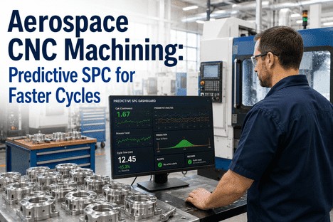
What the Dashboard Shows When Limits Adapt in Real Time
The adaptive control limit dashboard gives the supervisor a view that no static SPC chart can provide: the relationship between the current control boundary, the process centreline, and the tolerance limit — updated with every part, with a clear indication of whether the current limit state is stable, tightening, or widening.
Active Band Display
The current UCL and LCL are displayed as a shaded band on the control chart, with the tolerance limits shown as reference lines. The gap between the control limit band and the tolerance band is the operating margin. When adaptive limits tighten during stable periods, the band shrinks and the margin widens — the supervisor sees that the process has room to absorb variation before reaching the tolerance boundary. When limits widen during warm-up or batch changes, the band expands and the margin narrows — the supervisor sees that the process is in a period of expected higher variation and no action is required unless the band reaches the tolerance line.
Limit Change Log
Each time the adaptive engine adjusts a control limit, the event appears in a timeline panel on the dashboard. The entry shows the feature, the previous limit value, the new limit value, the rolling data window that drove the change, and the classification (common-cause adjustment or assignable-cause event). The supervisor reviews the change log at the start of each shift to understand what the process has done overnight — which limits have moved, why they moved, and whether any action is required based on the magnitude or frequency of adjustments.
False Alarm Counter
A live counter on the dashboard tracks the number of false alarms avoided by the adaptive limit engine since deployment. Each time a static limit would have fired a false alarm, the counter increments and records the feature, the condition (warm-up, batch change, transient spike), and the static limit value that would have triggered the alarm. This gives the supervisor and plant management a direct metric of the improvement in control chart reliability — not a theoretical estimate, but a count of actual false alarms that were suppressed because the limits adapted to the real process state.
Before Adaptive Limits — Static SPC
Operators see 12–18 OOC signals per shift. They have learned to ignore the first 10 because 8 of them will be false alarms. By the time a real signal appears, the operator's default response is to check the next part rather than stop and investigate. The static chart has lost its authority through accumulated false positives. The process runs without effective control because the control chart has been discredited by its own limits.
After Adaptive Limits — Dynamic SPC
Operators see 2–4 OOC signals per shift. Every one is a real event requiring investigation. The adaptive chart has earned its authority through consistent accuracy. When an alarm fires, the operator stops immediately because the history shows that the adaptive limit only fires on verified assignable-cause events. The false alarm rate has dropped 70%. The operator trusts the chart. The chart controls the process.
Deploying Adaptive Control Limits: The First 60 Days
The deployment of adaptive control limits follows a structured path designed to build confidence through direct comparison. The supervisor and operator teams see the adaptive limits running alongside the static limits for 30 days before the adaptive model becomes the primary control source.
Weeks 1–2
Baseline and Configuration
Historical process data loaded. Adaptive limit engine initialised on past 90 days. Dashboard configured with side-by-side static and adaptive limit views. Supervisor team trained on interpretation in a single 60-minute session.
Weeks 3–4
Parallel Validation
Both limit models run simultaneously. Every adaptive limit adjustment is compared against the static limit behaviour for the same data. False alarm rate reduction documented. Operator team provides feedback on alert accuracy and trust levels.
Weeks 5–6
Live Activation
Adaptive limits become primary control source. Static limits retained as background reference. False alarm rate target confirmed at 70% reduction. Limit change log activated. First AS9100 audit with adaptive limit documentation reviewed.
Weeks 7–8
Optimisation and Scale Planning
30-day adaptive limit performance analysed. Feature-level tuning applied for optimal window sizes and EWMA parameters. Results documented for replication planning to additional cells. Operator trust survey completed.
Conclusion
Fixed control limits on aerospace CNC SPC charts have a single, irreparable flaw: they describe the process that existed during the capability study, not the process that is running on the floor today. As tools wear, material batches vary, coolant concentrations shift, and fixtures age, the gap between the static control boundary and the real process boundary widens. The result is a chart that generates false alarms during normal operation, misses real signals during critical drift periods, and gradually loses the trust of the operators and supervisors who depend on it for quality decisions.
Adaptive control limits close this gap by recalculating UCL and LCL dynamically against a rolling window of current production data. The limits tighten when the process narrows, providing earlier detection of tool wear onset. They widen when natural variation increases, eliminating false alarms during warm-up and material batch changes. Every adjustment is classified by pattern — common-cause shifts adjust the limits, assignable-cause trends trigger alarms, transient noise is ignored. And every limit change is logged with full traceability for AS9100 audit compliance.
iFactory's adaptive control limit platform is built for aerospace CNC machining supervisors who need an SPC chart that describes the process as it is, not as it was. Book a Demo to see adaptive limits running on a CNC machining use case matched to your production profile, or talk to an expert about deploying adaptive control limits on your first cell and measuring the false alarm reduction in the first 30 days.
Frequently Asked Questions
No. The adaptive engine widens limits only for known, classified states — warm-up periods after startup, material batch changes, and transient events that the system has learned are part of normal operation. The widening is bounded by the tolerance limit. The adaptive limit never expands beyond the specification boundary. For periods of legitimate assignable-cause drift — tool wear progression, fixture displacement, coolant system failure — the limits tighten, not widen, because the rolling window detects the increasing variance and responds with a control boundary that is more sensitive, not less. The distinction between widening for known common-cause states and tightening for unknown assignable-cause trends is the core of the adaptive algorithm. It does not trade detection sensitivity for false alarm reduction. It eliminates false alarms by recognising which variation is expected and which is not. Talk to an expert about configuring the adaptive window sizes and classification thresholds for your cell.
The adaptive engine detects the tool change event through the combination of a step-change in the process mean and a reduction in variance. The first 2–3 parts after a tool change typically show a tighter distribution and a shifted centreline compared to the last parts on the previous tool. The adaptive algorithm classifies this as a common-cause event (tool replacement is a scheduled production event, not an anomaly) and recalculates the control limits to the new-tool baseline. The transition is typically complete within 5 parts — faster than the rolling window's full length because the EWMA weighting assigns higher priority to the most recent data points. During these 5 parts, both the old limits (wider, from the worn-tool state) and the new limits (tightening, to the new-tool state) are visible on the dashboard, so the operator sees the convergence. No false alarm fires during the transition because the adaptive engine recognises the pattern as a scheduled tool change, not a process failure. Book a Demo to see the tool change transition visualised on the control chart.
Every adaptive limit adjustment generates an auditable record containing: timestamp, machine identifier, feature identifier, previous UCL and LCL values, new UCL and LCL values, the rolling data window size that drove the change, the classification of the event (common-cause or assignable-cause), and the statistical method used for the recalculation (rolling standard deviation, EWMA parameter state, or pattern classification result). This record is stored in the AS9100 documentation repository alongside the part-level inspection results. During an audit, the quality engineer exports the limit change log for any date range and cell in under one minute. The auditor sees a complete chain of control limit adjustments with the process data that justified each change. This eliminates the documentation gap that occurs when static SPC limits are set during a capability study and then operated without recalculation for months or years — producing a situation where the control limits in use have no documented rationale connecting them to the current process state. Talk to an expert about the AS9100 documentation output configured for your quality management system.
Yes. The adaptive limit engine can replay historical production data with adaptive limits applied retrospectively. This is typically done during the baseline and configuration phase to establish the expected false alarm reduction before deployment begins. The retrospective analysis processes the last 90 to 180 days of historical measurement data through the adaptive algorithm and produces a comparison report: for each feature and machine, it shows how many OOC signals the static limits generated, how many of those were false alarms (verified against the quality record), how many the adaptive limits would have generated, and the net improvement in signal-to-noise ratio. This report is used to calibrate the adaptive window sizes and EWMA parameters before live deployment, and it provides the supervisor team with a data-driven expectation of the improvement they will see in the first 30 days of parallel validation. The retrospective analysis does not require any production disruption — it runs on archived data, independent of the live production system. Book a Demo to see a retrospective analysis for your own historical production data.
The adaptive limit engine includes a minimum limit width guard that prevents the control boundary from contracting below a configurable floor. This floor is set at 60% of the static control limit width established during the capability study, ensuring that even during extended periods of extremely stable operation, the adaptive limits retain sufficient sensitivity to detect a sudden disturbance without generating false alarms from normal random variation. Additionally, the EWMA weighting mechanism provides a natural buffer: a sudden disturbance produces a large deviation in the current data point compared to the rolling window, and the EWMA statistic amplifies this deviation because the recent data receives the highest weight. The result is that an unexpected disturbance is detected faster by an adaptive limit that has tightened during a stable period than by a static limit that has remained at a fixed width throughout the same period. The minimum width guard ensures that the adaptive limit never becomes so narrow that normal random variation triggers false alarms, but the normal adaptive narrowing during stable periods consistently improves detection speed for real disturbances. Talk to an expert about configuring the minimum limit width guard for your specific process risk profile.
Your Control Limits Are Telling You About a Process That No Longer Exists. Adaptive Limits Show You What Is Happening Right Now.
iFactory's adaptive control limit platform replaces static UCL/LCL with self-adjusting boundaries that follow the real process — delivering a 60–70% reduction in false alarms, 3–5x faster shift detection, and AS9100-compliant limit change logs generated automatically on every cell.