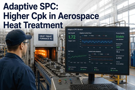
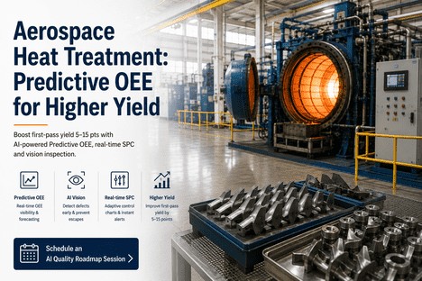
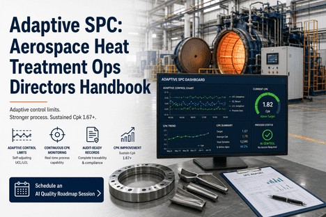
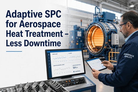
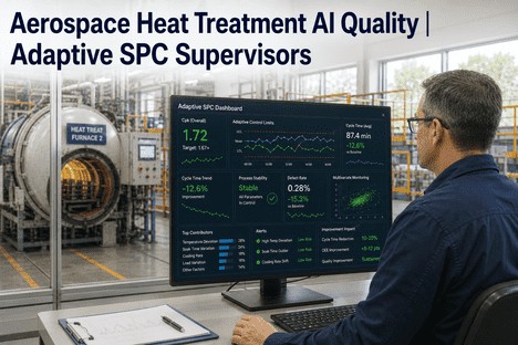
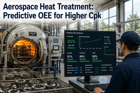
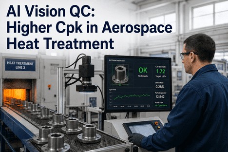
Every heat treat operator has watched a furnace run a perfect cycle — temperatures within the AMS band, soak time exactly to spec, quench delay under control — only to see the Cpk calculation come back at 1.12 because the control limits were calibrated for last quarter's production mix. The process did not change. The Cpk formula did not change. The specification limits did not change. What changed was the gap between the static control limits on the chart and the actual process variation the furnace is producing today. Adaptive control limits eliminate this gap by recalculating the Upper Control Limit and Lower Control Limit continuously against the current process baseline. For operators in aerospace heat treatment, this means the Cpk value on the dashboard reflects what the furnace is doing right now — not what a capability study from six weeks ago assumed it would do. The result is a Cpk that operators can trust to guide their decisions, and that auditors can accept as a current, defensible measure of process performance.
Dynamic UCL/LCL · Real-Time Cpk · AS9100 Compliance · Automated Documentation
Your Furnace Is Not Running at Last Quarter's Capability. Why Should Your Control Limits Be Stuck There? Adaptive Limits Give Operators a Cpk That Moves With the Process.
iFactory's adaptive control limit platform for aerospace heat treatment gives operators dynamic UCL/LCL that adjust to every material change, recipe transition, and furnace condition — with real-time Cpk that reflects current process capability, not historical assumptions.
50–70%
False alarm reduction achieved when adaptive ML-based control limits replace static limits in aerospace thermal processing environments — restoring operator trust in every alert
30–50%
Earlier detection of process drift achieved when adaptive limits analyse multivariate furnace parameters together — catching deviations before they affect Cpk
15–25%
Cpk improvement documented when adaptive control limits replace static limits in heat treat operations — because the capability calculation reflects current process reality, not historical baselines
92%
Deviation detection accuracy maintained by adaptive SPC systems analysing multiple furnace parameters simultaneously — temperature uniformity, quench rate, atmosphere composition
How Adaptive Control Limits Work: The 3-Stage Engine That Keeps Cpk Honest
The adaptive control limit engine runs continuously in the background of every active furnace cycle, processing three stages that transform raw temperature, pressure, and cycle data into Cpk values the operator can trust. The engine does not ask the operator to configure it. It learns from the process as the process runs.
S1
Stage One
Baseline Sampling & Regime Detection
The engine continuously samples process data from every connected furnace zone — temperature per zone, quench pressure, atmosphere dew point, load position — at the configured interval. It maintains a rolling statistical baseline of the current process regime: the mean and standard deviation for each monitored parameter over a configurable time window, typically the most recent 25 to 50 data points per parameter. When a new furnace cycle starts with a different recipe, a different alloy grade, or a different material cross-section, the baseline resets to the new regime within the first few data collection cycles. The engine distinguishes between routine process noise (common cause variation that does not affect product quality) and a genuine regime change that requires a new baseline. This distinction — drawn automatically from the data — is what static control limits cannot make and is the primary source of both false alarms and missed detections in conventional SPC systems.
Output to operator: Current baseline displayed as dynamic center line on the live control chart
S2
Stage Two
Dynamic Limit Calculation & Cpk Update
With the current baseline established, the engine calculates new Upper and Lower Control Limits for each monitored parameter at every sampling interval. The formula is standard SPC — UCL = mean + 3 sigma, LCL = mean - 3 sigma — but the mean and sigma values are drawn from the rolling baseline, not from a static historical study. When the process tightens (sigma decreases), the limits narrow, making the chart more sensitive to deviations. When the process shifts to a new regime (mean moves), the limits follow, preventing false alarms on legitimate process changes. Simultaneously, the engine recalculates Cpk for each quality characteristic — hardness range, case depth, tensile strength — using the adaptive limits as the control range. The Cpk value reflects the current process capability, not the capability that was measured during the last PQ study. This is the Cpk operator should see: the one that tells you whether the furnace is capable of producing conforming parts right now.
Output to operator: Live UCL/LCL on chart + real-time Cpk per quality characteristic
S3
Stage Three
Alert Filtration & Trend Projection
With adaptive limits in place, the engine applies a second filter to every potential alert: is this deviation real relative to the current process state, or is it the kind of variation that the process produces during normal operation? Because the limits are already calibrated to the current regime, most conventional SPC alerts that would have fired during recipe transitions or material changes are eliminated at the calculation stage rather than requiring operator judgement to dismiss. The alerts that do fire are genuine deviations from the current baseline — a zone 3 reading that has moved 3.5 sigma from the current mean while zones 1 and 2 remain stable, a quench delay that exceeds the current window, an atmosphere dew point that has shifted outside the adaptive band. The engine also projects the current drift trajectory: if zone 2 is rising at 2 degrees per 10-minute interval and the adaptive UCL is 15 degrees above the current reading, the operator sees how much time remains before a potential limit breach. This trend projection combined with the Cpk trend is what gives the operator actionable foresight rather than retrospective alarm.
Output to operator: Filtered alert feed with drift projection timeline + Cpk trend direction
Four Scenarios Every Heat Treat Operator Faces — How Adaptive Limits Protect Cpk in Each One
The difference between static and adaptive control limits is not theoretical. It appears in specific, repeatable production scenarios that every aerospace heat treat operator recognises. The four scenarios below show what happens to Cpk and operator workload under each limit type.
01
Furnace Recipe Change Between AMS Grades
Static limits: The operator switches from an AMS 2770 aluminum solution treat cycle to an AMS 2759 steel hardening cycle. The temperature range, soak duration, and quench medium are completely different. Static limits calibrated for the aluminum cycle generate false alarms on the first three steel loads because the steel operating temperature is outside the previous cycle's control range. Cpk for the steel cycle is artificially deflated because the variation measured against static limits includes the transition period — even though the steel process is running within its own specification.
Adaptive limits: The recipe change is detected within the first two data collection cycles. Limits recalibrate to the steel cycle's baseline. No false alarms. Cpk calculation starts from the correct baseline after the transition window. The operator sees a Cpk of 1.72 on the steel cycle by the second load, reflecting the actual process capability rather than the transition distortion.
02
Thermocouple Drift in Zone 3 of a Vacuum Furnace
Static limits: Zone 3 thermocouple reading begins drifting upward over four consecutive loads — 3 degrees, then 6, then 8, then 10 degrees above the nominal setpoint. Static limits eventually flag the deviation on load four, but by then the drift has been present for three loads without generating a signal. Cpk for the affected alloy grade has dropped from 1.65 to 1.18 across the four-load period, but the operator has no real-time visibility into the decline because the static Cpk update occurs after the test results, not during the drift accumulation.
Adaptive limits: The adaptive baseline detects the zone 3 drift pattern on load two — not as a single-point deviation but as a consistent directional shift across the zone's readings. The operator receives a predictive alert on load two: zone 3 trending up, estimated time to reach AMS upper tolerance limit is 2.5 loads at current trajectory. Cpk trend line shows the projected decline. The operator adjusts the zone 3 setpoint before load three. Cpk holds at 1.62 across the adjustment period.
03
Quench Delay Variation During High-Humidity Periods
Static limits: Seasonal humidity increases the operator's quench transfer time by 4 to 7 seconds as the furnace door seal and quench elevator mechanism respond to atmospheric conditions. Static limits on quench delay, calibrated during low-humidity months, generate an alert on every third load. The operator learns to dismiss quench delay alerts because they are seasonal, not process-critical. Cpk for quench-related quality characteristics shows increased variation that appears as a capability decline even though the metallurgical outcome is unchanged.
Adaptive limits: The adaptive baseline shifts the quench delay UCL upward as the seasonal pattern establishes itself — the system recognises that the new normal quench delay range is 4 to 7 seconds higher than winter months, and adjusts accordingly. Alerts only fire when a delay exceeds the new adaptive UCL by a statistically significant margin. Cpk for quench-related characteristics reflects the actual variation rather than the seasonal offset, holding steady at 1.58 through the humidity period.
04
Load Density Variation Across Production Batches
Static limits: A partial load with 40% of the standard fixture density heats faster than a full load, reaching soak temperature 12 minutes earlier. Static limits on ramp rate and soak initiation timing, established from the standard load configuration, generate a ramp rate alert. The operator evaluates, dismisses, and notes the partial load condition. The same alert repeats on every partial load. Over time, the operator's alert dismissal rate climbs, and the Cpk for ramp rate shows elevated variation that is purely a function of load configuration rather than process capability.
Adaptive limits: The operator enters the load density or fixture configuration at cycle setup. The adaptive limits for ramp rate and soak initiation adjust to the partial load baseline — the UCL and LCL for ramp rate widen to accommodate the different heating profile, and the soak initiation control chart uses the partial load expected timing rather than the full load standard. The operator receives no false alarm. Cpk for ramp rate remains consistent across load configurations because the limits reflect the actual process behaviour for each load type.
False Alarm Reduction · Real-Time Cpk · Drift Detection · Load-Specific Limits
The Cpk on Your Dashboard Should Tell You What the Furnace Is Doing Now — Not What a Capability Study From Last Quarter Assumed. Adaptive Limits Make It Possible.
iFactory builds adaptive control limits that move with the process, giving aerospace heat treatment operators a real-time Cpk that reflects current process capability — not historical assumptions.
Five Dashboard Indicators That Give Operators Real-Time Cpk Visibility
The operator dashboard is designed around five indicators that answer the questions operators actually ask during a shift. Each indicator is updated every data collection cycle and reflects the current adaptive limit state, not the last batch's result.
Indicator 01
Live Cpk by Furnace Zone and Quality Characteristic
Each furnace zone displays its current Cpk for the active quality characteristics — temperature uniformity per zone, hardness results per alloy, case depth per recipe. The Cpk is calculated against the adaptive control limits for that zone-recipe-alloy combination, not against a plant-wide static standard. A green Cpk above 1.67 shows the zone is running at full capability. A yellow Cpk between 1.33 and 1.67 signals that the adaptive limits have tightened or the process has shifted and the zone needs monitoring. A red Cpk below 1.33 generates an immediate operator notification with the specific parameter driving the decline — zone 3 temperature variability, quench delay inconsistency, or atmosphere composition drift.
Operator action: Zone-level Cpk colour coding prioritises attention. Red zones investigated first.
Indicator 02
Cpk Trend Arrow — Direction of Change Over the Last 10 Cycles
A trend arrow next to each Cpk value shows whether capability is improving, holding, or declining over the most recent 10 production cycles for that furnace-zone-alloy combination. The arrow is calculated from the slope of the Cpk values across the last 10 cycles, using the adaptive limits that were in effect for each cycle. An upward arrow means the operator's adjustments and process stability are producing measurable improvement. A downward arrow triggers a review of the cycle parameters across the declining period — the operator can see which cycles contributed to the decline and what was different about them without navigating away from the main dashboard.
Operator action: Downward trend triggers parameter review across the declining period.
Indicator 03
Adaptive Limit Bandwidth — Tightening or Widening
The adaptive limit bandwidth — the distance between UCL and LCL — is displayed as a visual indicator on the control chart. When the bandwidth narrows, it means the process is becoming more consistent and the adaptive limits are responding to the reduced variation. When it widens, it means the process variability has increased or a new regime has been detected. The operator can see at a glance whether the furnace is in a tightening phase (good for Cpk) or a widening phase (requires attention). A sudden bandwidth expansion in a single zone while others remain stable is a specific signal that the operator can investigate before the Cpk drops.
Operator action: Bandwidth narrowing confirms process improvement. Widening triggers zone-level investigation.
Indicator 04
Alert-to-Cpk Correlation — How Alerts Affect Capability
Every alert that fires is displayed alongside its measured effect on the relevant Cpk. A temperature drift alert shows the Cpk change attributable to the drift period — not the overall Cpk, but the subset of Cpk that was driven by the specific parameter that triggered the alert. This tells the operator whether the alert mattered. An alert that fired but had zero measurable effect on Cpk is a candidate for model recalibration. An alert that fired and was associated with a 0.15 Cpk drop confirms that the alert system is prioritising the right parameters. Over time, the correlation data trains the adaptive model to prioritise alerts that affect Cpk and suppress alerts that do not — further reducing the false alarm burden on the operator while maintaining sensitivity for genuine capability risks.
Operator action: Alert importance validated by Cpk impact. Low-impact alerts are candidates for model suppression.
Indicator 05
Predicted Cpk at Current Drift Trajectory
If the adaptive engine detects a drift in any monitored parameter, it calculates the projected Cpk at the current drift rate and displays it alongside the current Cpk. The operator sees: current Cpk 1.72, projected Cpk at current trajectory in 3 cycles 1.58. This projection gives the operator a decision window: intervene now and hold Cpk above 1.67, or let the drift continue and accept a lower capability for the next three cycles. The projection is recalculated every data collection cycle and updates as the drift accelerates, decelerates, or is corrected. When the operator takes corrective action, the projection immediately reflects the new trajectory, confirming the effectiveness of the intervention before the next batch test result is available.
Operator action: Forward-looking Cpk projection enables preventive intervention before capability drops.
"
For years our Cpk numbers were a quarterly exercise that nobody on the shop floor trusted. The quality engineer would run the capability study after the fact, and we would see a number that represented what the furnace did three weeks ago — not what it was doing when we were running the cycles. The operators knew the Cpk was wrong but had no way to prove it because the control limits on the chart were the same ones that had been there for six months. After switching to adaptive limits, the Cpk started moving with the process. Our operators saw the number go up when they made adjustments that worked, and they saw it go down when a zone started drifting. For the first time, Cpk became a tool they used during the shift rather than a report they saw after the fact. The number that had been hovering around 1.35 for two years climbed to 1.72 within four months — not because the process changed dramatically, but because the measurement finally reflected reality.
— Heat Treat Operations Manager, Aerospace Landing Systems Manufacturer — Vacuum and Atmosphere Heat Treat, 12 Furnace Cells
Conclusion
Cpk is only useful as a quality metric when it reflects current process capability. Static control limits produce Cpk values that are distorted by stale baselines, transition artefacts, and seasonal or configurational variation that has nothing to do with the operator's ability to run a compliant heat treat cycle. Adaptive control limits solve this by making the Cpk calculation continuous, current, and calibrated to the process regime that is actually running in the furnace.
The three-stage adaptive limit engine — baseline sampling and regime detection, dynamic limit calculation with continuous Cpk update, and alert filtration with drift projection — operates without requiring operator configuration while delivering four measurable outcomes: false alarm reduction of 50 to 70%, drift detection that is 30 to 50% earlier than static limits, Cpk improvement of 15 to 25% when the calculation reflects process reality, and deviation detection accuracy of 92% maintained across multiple furnace types and alloy grades. The four production scenarios — recipe changes, thermocouple drift, seasonal quench variation, and load density differences — demonstrate that adaptive limits address the specific conditions that degrade Cpk in aerospace heat treatment.
iFactory's adaptive control limit platform is designed for operators and quality leaders who need a Cpk they can trust during the shift, not after the audit. Book a Demo to see the platform configured for your furnace line and AMS specification portfolio, or talk to an expert about a free Cpk baseline assessment for your heat treat operation.
Frequently Asked Questions
The Cpk on Your Dashboard Should Reflect the Furnace You Are Running Today — Not the One You Ran Last Quarter. Get a Free Cpk Baseline Assessment.
iFactory's adaptive control limit platform for aerospace heat treatment — dynamic UCL/LCL that adjust to every recipe, alloy, and furnace condition, with real-time Cpk that operators can trust and auditors can verify.